
Intro to R
24/01/2019
😎 What is R?
R - is a statistical programming language.
1
Programming language:
- new words: main commands;
- new grammar: rules of conjugation, punctuation;
- stylistic issues: conventions;
- dialects, for example
tidyverse.
2
Language is used for communication:
- with R environment,
- with external software,
- with websites, databases, messengers, etc.,
- with other researchers.
3
Statistical language
- first and main use of R is
statistical modelsand data management; - data collection, text processing, automated reports generation, web applications, data visualization;
- other uses are possible, but not recommended.
Base R and packages
R consists of many modules, or packages:
- base R, which is R itself, environment that accepts a set of basic commands and gives response;
- R packages, optional extensions of R, usually written in R language, that can be used right from inside R, but require separate installation.
a) Base R
- Installed initially, includes several essential packages,
- Only basic commands, such as
mean,sort,cor,lm(linear model).
b) R packages
- In practice you need tens of packages.
- Packages are independently developed by statisticians or other individuals.
- Most packages are stored in Comprehensive R Archive Network (CRAN), Bioconductor (mostly for genetics), or at the individual repositories, such as GitHub or GitLab.
- More than 13,000 R packages; most of them are regularly updated.
- Every R package has a specific set of purposes (or just a single), solves a speicific problem. For example, package
GPArotationprovides various methods of factor rotation, in exploratory factor analysis. - Many packages solve same problems, in different ways. Choosing the right R package is one of the tricky new tasks - check https://www.rdocumentation.org/taskviews .
- Most packages depend on other packages.
- (Almost) all packages have an open code, everyine can see what exactly happens under the hood.
- No more “black box” procedures.
Essential helpers
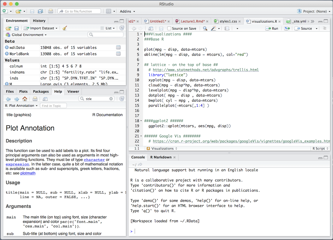
RStudio
RStudio - is an integrated development environment that facilitates programming. Needs to be installed after installing R.
❗️There is a trial online version: https://rstudio.cloud/ - very slow though.
alt text
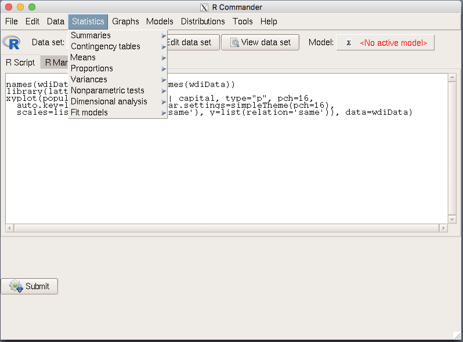
R commander 🐥
- SPSS-like interface that helps to create R code.
- http://www.rcommander.com/
- Recommended only for the very beginning.
- It is just another R package.
Installation and use of packages
install.packages("readxl") # Run once on the same machine
library("readxl")          # Run after every restart of R
# By the way, hashtag is used to comment R code, it is not read as R
🏗 Building blocks of R
Objects
You may think of R as a smart calculator.
5+5[1] 10Upper field is input (by human), lower field is output (by R).
[1] in output means a sequential number of value.
In addition to computation, R can store different data, every piece of data is called “object”. Every object has a name.
❗️Object names should begin with a character (not a number!).
❗️R differentiates between UPPER and lower case. (For ex., Mydata and mydata are treated as two different objects).
Kinds of objects (classes)
Objects can contain any information: numbers, texts, arrays of texts and numbers, tables, images, functions, other objects, etc.
a) Main kinds of variables
Functions that read data in, try to identify the type of the variable automatically, but it is better to check each variable’s class manually. To know the class, or structure of object, use str().
numeric
[1] 1.10 2.50 3.23 4.00 5.00numeric are used for continuous variables;
string/character
[1] "cat" "dog" "mouse"string or character for text variables;
factor (unordered)
[1] horsebean horsebean horsebean
Levels: casein horsebean linseed meatmeal soybean sunflower
so called factor are for nominal or
ordered factor
[1] Primary Primary
Levels: Primary < Secondary < Higher
ordinal (ordered factor) variables
logical
[1] FALSE TRUE TRUE TRUElogical can take only TRUE or FALSE values.
b) Structures of data storage
- vectors, created by
c()for separate variables; - flat (two-dimensional, SPSS or Excel-like) tables
data.framemost often used table of data; matrix- also two-dimensional, often used for matrix manipulations,array- multidimensional tables, for example, 3-dimensional or layered table,list- can contain different kinds of data, or other lists.
You can give names to each element in the data structures.
Each object can be created manually with a function of the same name:
vectors c()
c(1,2,3) # 'c' stands for "concatenate", it puts together several values and coerces them to the same type.[1] 1 2 3data.frame
data.frame(
  height=c(145,203,169),
  first.name=c("Ana", "Boris", "Claire")
  )
height first.name
1 145 Ana
2 203 Boris
3 169 Clairematrix
     [,1] [,2] [,3] [,4] [,5]
[1,]    1    7   13   19   25
[2,]    2    8   14   20   26
[3,]    3    9   15   21   27
[4,]    4   10   16   22   28
[5,]    5   11   17   23   29
[6,]    6   12   18   24   30
array
, , 1

     [,1] [,2] [,3] [,4] [,5]
[1,]    1    4    7   10   13
[2,]    2    5    8   11   14
[3,]    3    6    9   12   15

, , 2

     [,1] [,2] [,3] [,4] [,5]
[1,]   16   19   22   25   28
[2,]   17   20   23   26   29
[3,]   18   21   24   27   30
list
$`the name of the first element`
[1] 1 2 3 4 5

$`the name is not required though`
[1] "a" "c"

[[3]]
[1] "Just a single string"
Operators
We can create objects by using operators. Two objects a and b are assigned values. Then, we can use object names instead of values to proceed with analysis:
a <- 5
b <- 6
a + b
[1] 11<-- assignementoperator, desired name should be on the left side, assigned value(s) on the right.=- same as<-, but under R conventions, it is not recommended for object assignements.==- checks if two values are equal (do not confuse with single=!).-,+,/,*,^- basic math operators.
Functions
Functions - are typical operations saved to objects, they are created in order to avoid repeating the same code multiple times.
Functions drive R.
For example, mean() computed mean, sd() - standard deviation, с() concatinates several values to vector converts them nto the same type.
c(1, 2, "R", "", 0)[1] "1" "2" "R" "" "0"In and Out
Every function has some input information, or arguments (for example, data) and output (for example, an estimated statistical model).
Function syntax
Most functions have the following form:
FUNCTION_NAME(argument1 = "default value 1",
              argument2 = "default value 2",
                ...)
Sometimes default values are not specified but required, such arguments should be specified by a user. For example, function c() does not have defalt values at all, every argument is a value.
Arguments
Function subset has three required arguments:
subset(x, subset, select) x- data to use in subsetting,subset- what observation of data x should be left (filtering variable),select- what variables of data x should be left.
Output
Functions return some value, prints something in the terminal, or draws a plot. Functions differ by what they return, it is usually specified in the Help documentation under section “Value”.
Usage of functions
Arguments
Values can be assigned to arguments using only = operator.
❗️In order to check equality use ==. For example: a == b returns TRUE or FALSE, whereasa = b assigns object a with whatever value b has.
If argument has a default value and we agree with it, the argument can be omitted. Names of arguments can be omitted too, however, their values should be stated strictly in the specific order (order is shown in Help).
 # These two lines are equivalent:
 subset(x = mydata, subset = age > 65, select = c("health", "income"))
 subset(    mydata,          age > 65,          c("health", "income"))
Spaces do not affect the functioning of R. Use spaces freely to format R code.
Output
In most cases you want to save a function output to an object:
 # This line saves subset of older repondents and only two variables into a new object named old.respondents:

 old.respondents <- subset(mydata, age > 65, c("health", "income"))
❗️If you don’t save an output into an object, it is printed in the console window and lost, you can’t access it anymore. It is sometimes convenient only when you need to see just a single number.
If you save the result into an object, nothing is usually printed.
✂️ Filtering and getting parts of objects
Indexing data.frame
Any kind of data object can be indexed. data.frame is indexed by rows and columns:
flat.table[ROWS, COLUMNS]To access the value stored in the first row and fifth column:
PT[1, 5][1] 110158Rows and columns may be accessed by their names as well. To return the first value of the variable “idno”:
PT[1, "idno"][1] 110158In order to access all the values in the variable, just omit the row specification (but leave the comma!):
PT[, "idno"]Equivalently, a variable in data.frame can be accessed by $ sign:
PT$idno
Subsetting
By line numbers
Useful operator colon : to create sequence of numbers:
1:5[1] 1 2 3 4 5To return five upper rows of data.from.spss data and only two variables idno и cntry:
PT[1:5, c("idno", "cntry")]By values
In order to filter rows/observations by values of some variable, it requires two steps.
Step 1. Create a filtering variable of the class logical.
Logical values can be created using == sign:
2 + 2 == 5[1] FALSEThe same can be done with a vector (variable):
c(1,2,1) == 2[1] FALSE TRUE FALSEFinally, to create a filtering variable that is TRUE for all females and FALSE for all males:
filter.female <- PT$gndr == 2 # double equality sign!

summary(filter.female)
Mode FALSE TRUE
logical 530 740 Step 2. Use the filtering variable at the row index:
portuguese.females <- PT[filter.female, ]The two steps may be combined in a single expression:
portuguese.females <- PT[PT$gndr == 2, ]Alternative: subset()
Equivalent result may be obtained with subset() function:
portuguese.females <-
  subset(
      x = PT,               #data
      subset = gndr == 2    #criteria of row selection
  )
Indexing of lists
Lists are indexed using double brackets.
To get the first element of the list: - one.list[[1]]
or, if the list elements have names, by its name:
one.list[["my.named.element"]]
analogously
one.list$my.named.element
If the list’s element is subsettable, it can be accessed directly. For example, if the second elelment is data.frame, one can return first ten rows of it:
one.list [[ 2 ]] [1:10, ]
by the same token, if the first element of the list is another list:
one.list[[ 1 ]] [[ 5 ]]- to get fith element of the nested list.
Variable names
Get names
Function names() returns a vector of names of an object elements:
names(PT)[1:10] [1] "name" "essround" "edition" "proddate" "idno" "cntry"
[7] "nwspol" "netusoft" "netustm" "ppltrst" Assign names
Variable names can be replaced by direct assignement of new names:
names(PT)[1:3] <- c("IDnumber", "ESSround", "Version")Spaces in names
❗️ Names can include spaces, but it’s safewr to keep them short and spaceless.
- If you already have names with spaces, you may index them by using backticks `, for example
PT$`ID number`orPT[, "ID number"]
Graphics
𝓡 Base R graphics: plot()
plot() is a generic function to build R base plots, that applies different methods depending on the class of the object in its arguments.
- plot.dendrogram()
- plot.factor()
- plot.formula()
- plot.function()
- plot.lm()
- plot.density()
- etc.
plot.factor
plot(PT$big.city)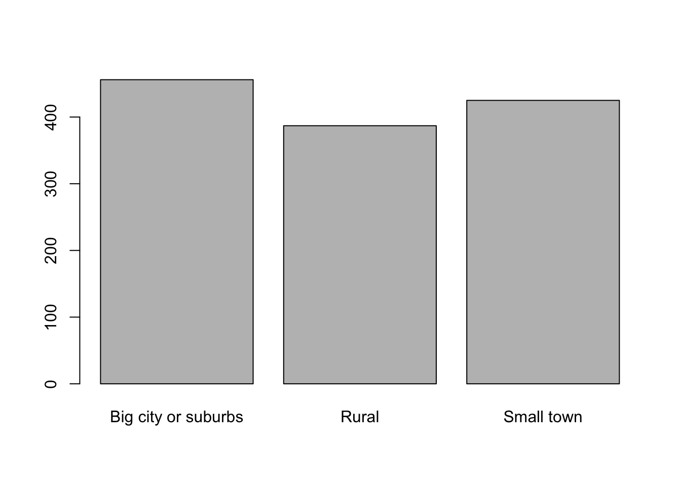
plot.xy & abline
plot(PT$agea, PT$eduyrs)
abline(17.7, -0.1463, col="red")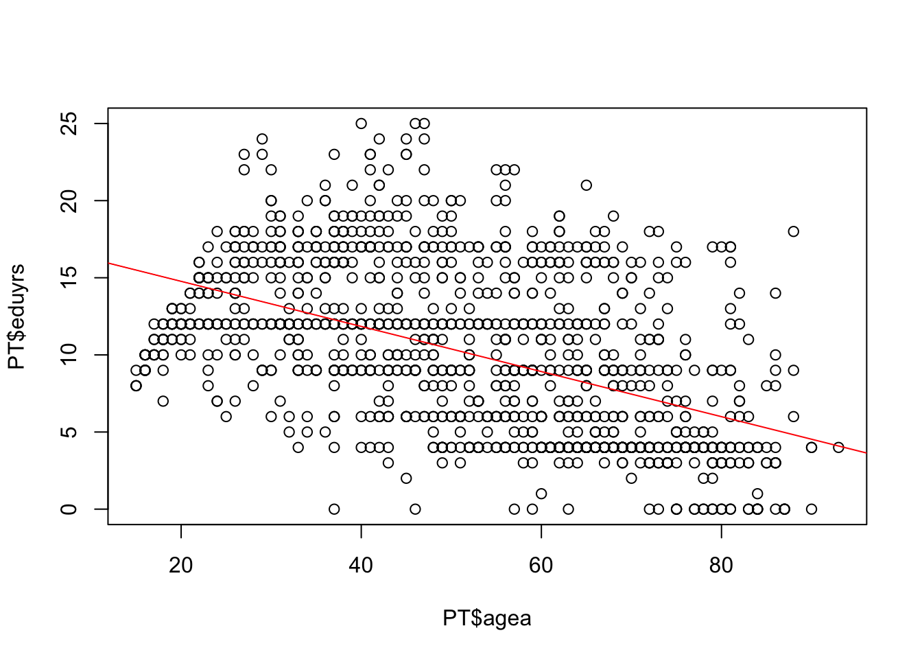
hist
hist(PT$eduyrs)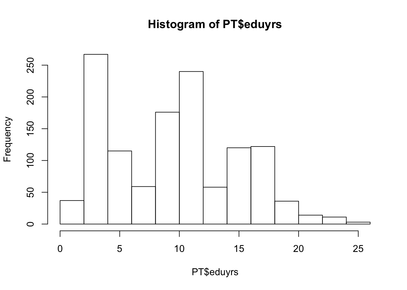
Lattice
xyplot() / dotplot()
library(lattice)
xyplot(eduyrs ~ agea | bigc, PT)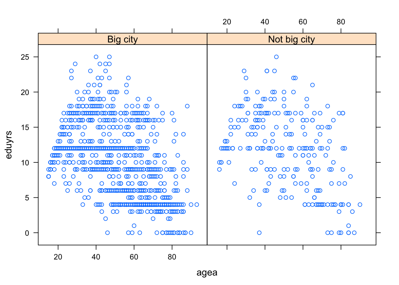
cloud()
library(lattice)
cloud(impfree.reversed ~ eduyrs*agea | bigc, PT)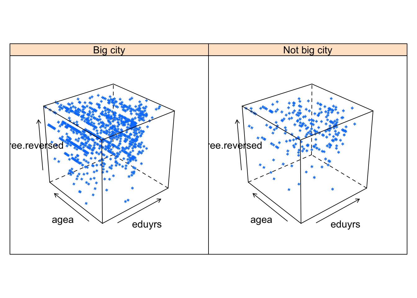
levelplot()
levelplot(eduyrs ~ agea*impfree.reversed, PT)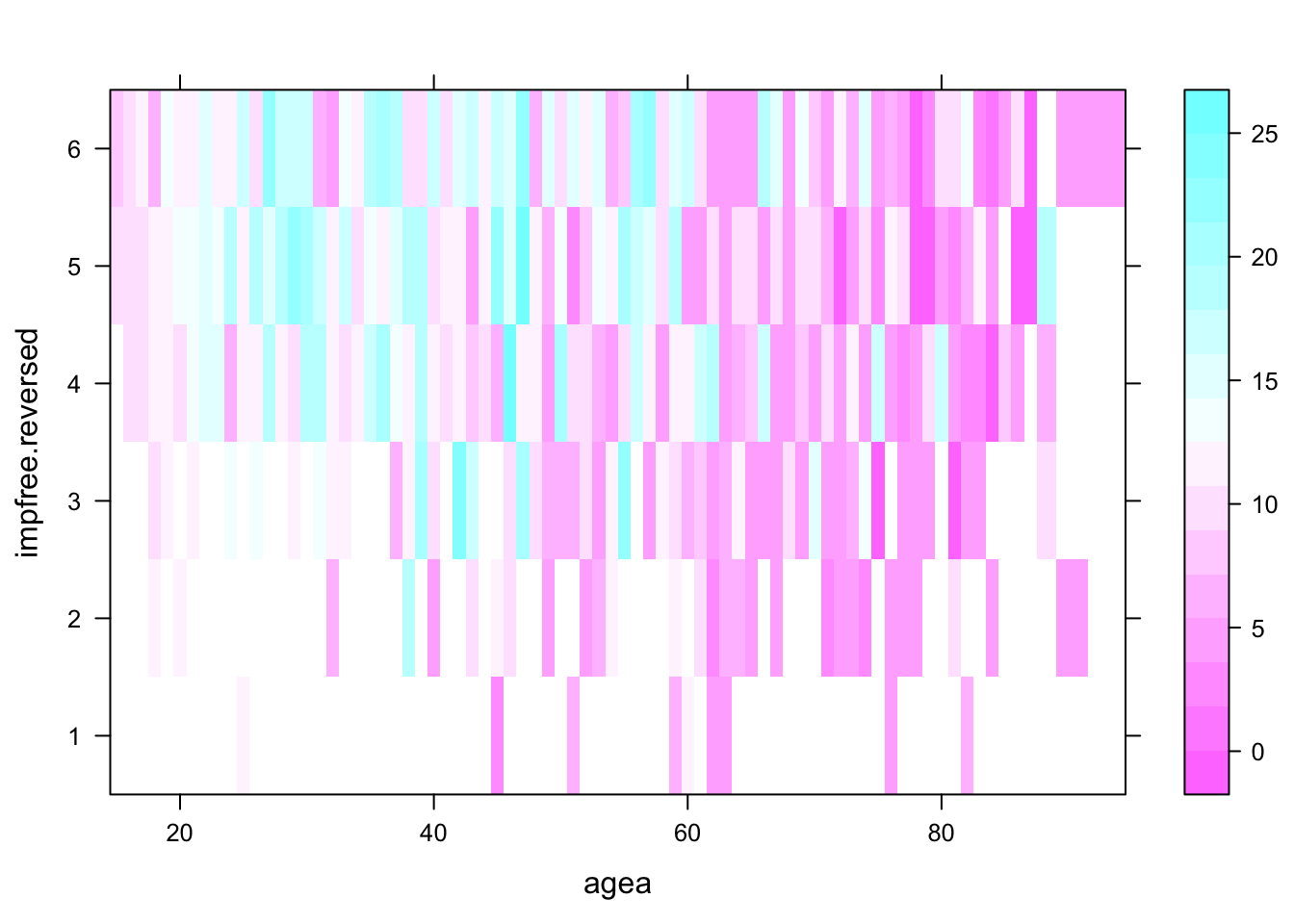
bwplot() - Box-whisker plot
library(lattice)
bwplot(eduyrs ~ big.city, PT, horizontal=FALSE)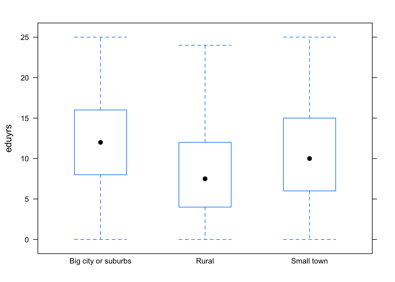
Whiskers - minimum (+1.5*IQR from the box), box - Q1 and Q3, median is the dot.
histogram()
histogram(as.vector(PT$eduyrs))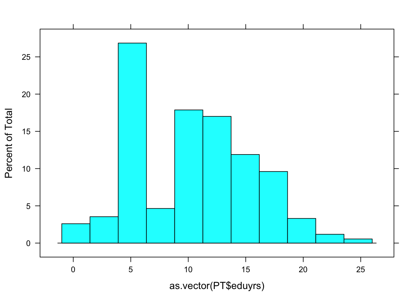
densityplot
densityplot(as.vector(PT$eduyrs))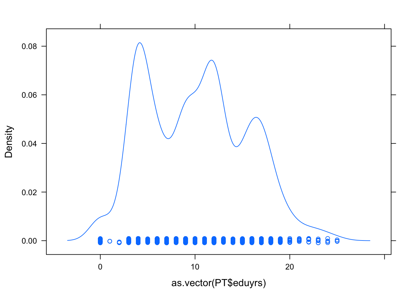
Many others
car Scatterplot
# Enriched scatterplot
library("car")
scatterplot(eduyrs ~ agea, PT)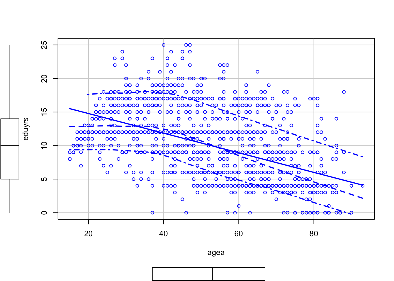
corrplot Correlation plots
#install.packages("corrplot")
library("corrplot")

corrplot(cor(PT[,501:511], use = "complete.obs")) 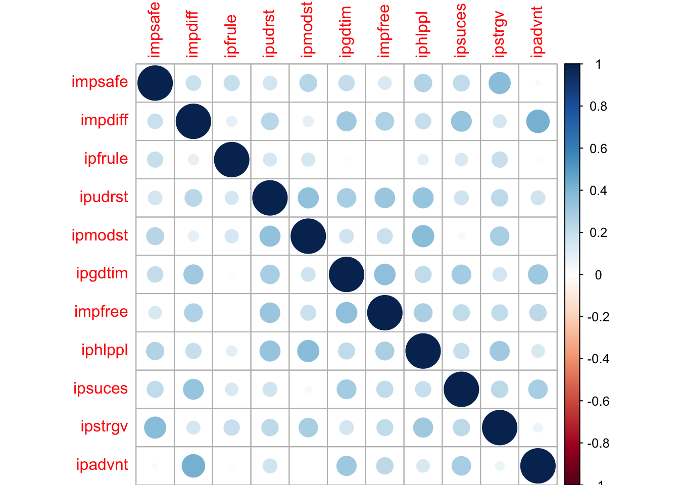
ggplot2
Next time!
Questions?
🐑 | 🐕 | 🐈 | 🐌 | 🐸 | 🐵