
Practical session 1. Read, recode, subset, describe, export
24/01/2019
1 Preliminary steps
1.1 Install R and Rstudio:
R: https://cloud.r-project.org/
RStudio: https://www.rstudio.com/products/rstudio/download/#download
1.2 Get aquainted with RStudio
- Examine all the windows and tabs in RStudio. Later, you can organize RStudio in your own way
- Set the working directory
setwd(), you can check it by usinggetwd()without arguments. - Create an R script file, File -> New file -> R script
2 ▶️ Play around
- Compute a sum of two numbers by entering in the Console window something like
4 + 100 - Create an R script file (File -> New file… -> R script).
- Write/copy the same command to the R script window and run it using either
 button or by combination Control+Enter on Windows or Command+Enter on Mac.
 - In the script window, create an object named
myVectorusingc()function, that contains numbers 1, 2, and 5. Run the line. Check if the object appeared in the Environment tab. If it did not, try one more time. - Multiply each element of the
myVectorobject by 10. Save the result in the object namedmyVector10. Check the result by printing the contents of themyVectorobject to the console. - Multiply only second element of the
myVectorobject by 10.
The correct codes are here.
3 📥 Read in the data
- Download data file ESS8PT.sav
- Move the data file into your working directory (get to know it by
getwd()or set it bysetwd()). - Read it in using
havenpackage. For this, you need to first install the package (install.packages()), then start it (library()), then use functionread_sav(). Save the read data in the object namedPT. Check if the created object appears in theEnvironmenttab. - Explore the structure of the data object by clicking on the
 button in Environment tab, or using function
 str().
The correct codes are here.
4 ☑️ Subsetting and filtering
4.1 Selection of observations
4.1.1 Play around
- Write code that returns observation 1 of the variable
ageain the datasetPT. - Print to the Console all the values of variable
agea. - Print to the Console all the variables of the third observation.
- Print to the Consople observations from 3rd to 5th of the variable
agea. - Save rows 5 to 10 of all variables to a new object called
subsetted.data.
4.1.2 Real-world task
Let’s select only female respodents, and clear out unnecessary variables, leaving only following:
- important to be free (
impfree), - age (
agea), - respondent’s type of settlement (
domicil), - years of education (
eduyrs).
We need to save a subset of data into a new object, naming it PT.females.
4.1.3 Way 1 - indexing
female.filter <- PT[ ,"gndr"] == 2

PT.females <-  PT[female.filter, c("impfree", "gndr", "eduyrs", "domicil", "agea")]

# or shorter

PT.females <-  PT[ PT$gndr == 2, c("impfree", "gndr", "eduyrs", "domicil", "agea")]
Check if the new object appeared in the Environment tab. How many observations does it have? How many variables?
4.1.4 Way 2 - subset
PT.females <- subset(
        x = PT,
        subset = gndr == 2, # select cases, use double equality sign  `==`
        select = c("impfree", "gndr", "eduyrs", "domicil", "agea") # select variables, `с()` merges several values into a vector
        )
4.2 Multiple filters
4.2.1 Boolean operators to create logical variables
x == 5Logical IS EQUAL. Returns TRUE when x equals 5 and FALSE in all the other cases.! xNOT (if x is TRUE, the expression returns FALSE, if x is FALSE, the expression returns TRUE).x & yLogical AND. If both x and y are TRUE, then outcome is TRUE. If one or both of them are FALSE, then FALSE is returned.x | yLogical OR. If x or y is TRUE, then TRUE is returned. Only if both are FALSE, this expression returns FALSE.
For example, to create a subset of females older than 60:
wom60 <- PT[ PT$gndr == 2 & PT$agea >= 60, ]Now, edit this line to create an object containing only three variables: eduyrs, domicil, impfree.
Remove this object from memory using rm() function, as we won’t need it.
5 🔣 Recoding
Let’s check the coding of the responses in the first variable impfree.
PT$impfree<Labelled double>: Important to make own decisions and be free
[1] 2 2 1 1 3 2 NA 3 3 2 3 1 1 3 1 2 2 1 4 1 2 3 1
[24] 4 2 1 3 NA 2 3 1 4 4 5 1 3 1 3 3 3 1 4 1 3 3 1
[47] 3 1 2 2 3 1 1 6 2 1 2 2 1 1 1 1 2 1 2 6 1 1 2
[70] 3 1 3 1 1 1 2 3 2 3 1 2 2 3 3 1 4 2 1 NA 4 1 2
[93] 3 1 1 2 3 5 1 3 2 2 4 2 2 1 1 2 3 1 3 4 1 1 2
[116] 4 3 1 3 2 2 1 1 1 3 2 2 2 2 1 1 3 2 1 2 1 3 2
[139] 5 2 3 2 3 1 2 2 2 2 2 1 5 3 1 2 3 2 3 1 4 3 4
[162] 3 2 1 3 2 3 5 1 3 2 2 3 1 3 3 1 6 2 3 3 2 2 3
[185] 4 2 2 1 2 3 1 1 3 4 1 1 2 3 3 2 2 3 3 3 3 3 1
[208] 2 4 1 1 2 3 3 2 1 1 3 1 1 3 1 3 2 2 5 3 3 3 1
[231] 3 1 4 1 1 3 3 3 1 1 4 2 3 2 2 2 1 2 1 1 2 3 2
[254] 2 2 2 1 1 2 3 1 1 1 2 2 3 3 2 NA 3 2 1 1 1 1 2
[277] 1 4 1 2 2 3 NA 1 1 1 1 1 3 3 2 3 2 1 1 4 1 3 2
[300] 3 2 2 3 3 3 3 3 5 1 1 3 2 3 1 3 2 3 3 1 3 1 3
[323] 2 3 3 1 4 2 1 4 2 3 2 1 5 1 1 1 4 2 4 1 3 1 2
[346] 1 4 4 3 1 1 2 5 3 2 3 1 2 2 3 1 1 3 2 5 1 1 2
[369] 3 1 1 3 3 3 3 2 1 1 2 2 2 1 3 1 1 2 1 3 3 2 2
[392] 3 2 3 3 2 4 1 1 NA 3 3 1 1 1 2 1 2 4 1 3 1 3 1
[415] 1 3 3 1 2 2 3 2 1 2 5 1 2 1 1 3 1 3 1 3 1 1 1
[438] 3 1 5 2 3 2 2 1 2 2 4 6 2 3 3 2 2 1 2 2 1 3 3
[461] 3 3 3 4 2 1 1 5 3 4 3 2 4 2 1 3 3 5 3 2 2 1 3
[484] 2 2 4 1 3 2 1 3 3 1 3 3 3 2 5 5 3 5 4 3 3 2 3
[507] 3 3 4 2 2 3 2 2 1 1 3 1 3 2 2 4 1 4 1 4 2 6 2
[530] 2 2 2 2 1 4 3 2 1 1 1 1 2 2 2 2 3 3 4 5 4 5 2
[553] 2 3 3 1 2 3 3 2 2 4 1 2 2 2 2 4 1 2 2 1 4 1 1
[576] 4 3 4 1 2 2 2 2 2 1 3 3 1 2 1 2 4 2 3 3 3 1 3
[599] 3 2 3 2 2 1 1 2 2 2 1 4 2 2 5 3 3 2 4 3 3 5 3
[622] 5 3 2 3 3 3 4 3 4 2 2 1 5 2 2 2 3 3 3 3 3 3 2
[645] 3 1 4 3 3 4 2 2 2 3 2 4 3 3 1 1 3 1 1 2 1 3 2
[668] 2 2 4 2 1 2 1 1 1 1 5 2 5 1 3 2 2 3 1 2 3 3 2
[691] 3 3 2 3 3 2 1 1 2 2 3 3 1 3 2 5 3 1 2 4 3 6 3
[714] 1 3 1 1 3 1 1 1 1 1 2 1 4 1 1 3 2 1 2 3 1 2 1
[737] 3 1 3 6 1 3 1 2 3 1 5 1 2 2 3 3 1 3 1 4 4 2 5
[760] 1 3 2 1 3 5 1 1 2 3 1 3 4 1 2 1 3 2 2 1 2 4 1
[783] 1 1 4 3 1 3 3 3 3 4 2 2 2 1 2 2 2 1 3 3 1 3 2
[806] 3 3 1 2 1 1 1 4 1 1 3 3 3 1 3 1 3 1 1 1 2 2 3
[829] 1 2 1 3 3 1 1 3 1 1 2 3 2 2 1 1 2 3 3 1 4 1 3
[852] 4 2 2 2 2 2 2 1 3 1 6 2 2 NA 3 1 3 1 2 1 1 2 4
[875] 1 3 2 3 1 1 2 3 1 1 2 1 3 1 3 2 2 2 NA 1 1 3 3
[898] 1 3 3 2 3 3 2 1 1 3 4 2 1 1 2 3 2 3 3 3 2 2 5
[921] 4 1 3 4 2 3 3 3 1 4 2 1 1 2 1 3 1 2 1 4 1 3 4
[944] 5 2 5 5 2 1 3 2 1 2 2 2 3 2 1 3 1 3 5 1 2 3 2
[967] 2 2 1 1 2 2 3 3 1 1 2 3 1 1 2 3 2 2 2 3 3 2 2
[990] 4 5 2 4 3 2 3 1 2 3 1 1 2 3 2 2 1 2 1 4 3 1 1
[1013] 2 1 1 4 3 2 2 2 2 3 1 3 3 3 3 1 1 3 1 1 2 2 3
[1036] 3 1 3 3 3 3 3 2 2 2 2 2 1 2 3 2 2 1 2 1 3 2 1
[1059] 1 3 1 4 3 5 1 1 1 3 1 2 1 1 3 2 1 3 1 3 3 2 2
[1082] 2 3 1 2 3 2 3 1 3 1 2 4 3 3 3 4 3 2 1 1 1 1 2
[1105] 3 1 2 3 1 1 1 1 2 1 1 1 1 3 1 3 3 2 3 4 2 1 1
[1128] 1 2 1 3 1 1 4 2 1 1 1 1 2 3 2 2 6 2 4 2 2 1 3
[1151] 2 1 2 1 3 3 3 1 3 2 1 1 1 3 4 3 4 4 2 2 2 3 1
[1174] 4 1 1 4 3 3 3 3 1 2 3 5 3 1 3 1 1 1 4 2 3 1 3
[1197] 3 1 1 2 3 2 3 2 2 3 6 3 1 5 1 3 4 1 2 NA 4 4 3
[1220] 4 2 3 3 3 1 3 3 2 4 2 2 2 1 1 1 2 1 2 3 1 3 3
[1243] 3 2 2 2 3 1 1 2 3 2 3 2 1 2 3 2 1 2 2 2 1 3 2
[1266] 4 2 3 3 3
Labels:
value label
1 Very much like me
2 Like me
3 Somewhat like me
4 A little like me
5 Not like me
6 Not like me at all
7 Refusal
8 Don't know
9 No answerFrom the Labels section we can see that the variable is reverse-coded. Thus, we need to recode it back.
5.1 Recode in car
If you don’t have it, install car package first. And then:
library("car")
PT$impfree.reversed <- Recode(
  var = PT$impfree,  # original variable
    recodes = "1=6; 2=5; 3=4; 4=3; 5=2; 6=1; NA=NA; else=NA", # recoding rules, follow pattern 'old value = new value'
  as.numeric=TRUE
  )
Let’s check if the recoding went well with cross-tabulation using table() function:
table(PT$impfree.reversed, PT$impfree)
      1   2   3   4   5   6
  1   0   0   0   0   0  10
  2   0   0   0   0  38   0
  3   0   0   0  94   0   0
  4   0   0 367   0   0   0
  5   0 367   0   0   0   0
6 385 0 0 0 0 0❗️Note that labels are not automatically recoded. In order to recode labels, use rec() function of sjmisc package.
Now recode domicil variable to a new three-category variable: (1) big city or suburbs, (2) small city, (3) village and farmhouse. Add an argument as.factor with value TRUE to acknowledge that it is a nominal variable.
library(car) # Start the `car` package

PT$big.city <- Recode(
  var = PT$domicil,  # original variable
  recodes =
    " c(1,2)  = 'Big city or suburbs';
      c(3)    = 'Small town';
      c(4,5)  = 'Rural'
    ",
  as.factor=TRUE   # signifies that the output variable is categorical nominal
  )
Use table() to check if the desired result achieved.
5.2 Optional: manual recoding
Recoding is possible with base R indexing tools.
5.2.1 Step 1. Create empty variable
PT$big.city <- rep(NA, nrow(PT)) # rep stands for repeat, nrow counts the number of rows, so that empty value "" is repeated as many times as there rows.Select observations which has value of domicil equal to 3 and filter the new empty variable, assigning them value “small town”.
PT$big.city[ PT$domicil == 3] <- "Small town"Likewise for other responses (| stands for logical “or”):
PT$big.city[PT$domicil == 1 | PT$domicil == 2] <- "Big city or suburbs"
PT$big.city[PT$domicil == 4 | PT$domicil == 5] <- "Rural"
We got a variable of class character, but it’s not a text variable. We need to change it to class factor:
PT$big.city <- as.factor(PT$big.city)And finally let’s check if recoding was successful:
table(PT$big.city, PT$domicil, useNA="always")
                        1   2   3   4   5 <NA>
  Big city or suburbs 256 200   0   0   0    0
  Rural                 0   0   0 359  28    0
  Small town            0   0 425   0   0    0
  <NA>                  0   0   0   0   0    2
6 📝 Descriptive statistics
Quick overview of descriptive statistics of all the variables in data set is handy with summary() function:
summary(PT.females) impfree gndr eduyrs domicil
Min. :1.000 Min. :2 Min. : 0.000 Min. :1.000
1st Qu.:1.000 1st Qu.:2 1st Qu.: 4.000 1st Qu.:2.000
Median :2.000 Median :2 Median : 9.000 Median :3.000
Mean :2.224 Mean :2 Mean : 9.881 Mean :2.797
3rd Qu.:3.000 3rd Qu.:2 3rd Qu.:14.000 3rd Qu.:4.000
Max. :6.000 Max. :2 Max. :25.000 Max. :5.000
NA's :7 NA's :8 NA's :1
agea
Min. :15.00
1st Qu.:38.00
Median :53.00
Mean :52.38
3rd Qu.:67.00
Max. :93.00
6.1 Cross-tabulation / contingency tables / frequencies
table():
table(PT$impfree.reversed,
      PT$big.city,
      useNA="always"
      )
       Big city or suburbs Rural Small town <NA>
  1                      5     2          3    0
  2                      9    15         14    0
  3                     29    40         25    0
  4                    131   126        110    0
  5                    129   100        138    0
  6                    151    99        133    2
  <NA>                   2     5          2    0
Important argument useNA="always", otherwise missing values are not shown at all.
To get proportions/percents prop.table(). Argument margin = NULL (defualt) returns proportion based on the total sum, 1 - proportion by rows, 2 - proportions by columns.
table1<- table(PT$impfree.reversed,
               PT$big.city,
               useNA="always"
               )

prop.table(table1,
           margin=2
           )
       Big city or suburbs       Rural  Small town        <NA>
  1            0.010964912 0.005167959 0.007058824 0.000000000
  2            0.019736842 0.038759690 0.032941176 0.000000000
  3            0.063596491 0.103359173 0.058823529 0.000000000
  4            0.287280702 0.325581395 0.258823529 0.000000000
  5            0.282894737 0.258397933 0.324705882 0.000000000
  6            0.331140351 0.255813953 0.312941176 1.000000000
  <NA>         0.004385965 0.012919897 0.004705882 0.000000000
At the next step, the numbers can be rounded
p.table <- prop.table(table1, margin=2)

round(p.table, 2)
       Big city or suburbs Rural Small town <NA>
  1                   0.01  0.01       0.01 0.00
  2                   0.02  0.04       0.03 0.00
  3                   0.06  0.10       0.06 0.00
  4                   0.29  0.33       0.26 0.00
  5                   0.28  0.26       0.32 0.00
  6                   0.33  0.26       0.31 1.00
  <NA>                0.00  0.01       0.00 0.00
6.2 Central tendency measures
Using mean() and sd(), compute means and standard deviations of variable impfree.
mean(PT$agea, na.rm=TRUE)[1] 52.04882mean(PT$impfree.reversed, na.rm=TRUE)[1] 4.743061sd(PT$agea, na.rm=TRUE)[1] 18.30046sd(PT$impfree.reversed, na.rm=TRUE)[1] 1.107962Now try to compute mean and standard deviation using functions sum(), length(), and var().
Correct codes are here
6.3 Group statistics and aggregation
When one variable is continuous and the other categorical, computing group means is meaningful.
Two of the many function for this: by() and aggregate().
aggregate(x       = PT$impfree.reversed, # continuous variable to be aggregated
          by      = list(PT$gndr),             # grouping variable
          FUN     = mean,                # aggregation function
          na.rm   = TRUE                 # remove NAs?
)
There can be more than one grouping variable:
aggregate(PT$impfree.reversed,
          by=PT[, c("big.city", "gndr")],
          mean,
          na.rm=TRUE
          )
Now we can compute standard deviations by replacing mean with sd:
aggregate(PT$impfree.reversed,
          by=PT[, c("big.city", "gndr")],
          sd,
          na.rm = TRUE
          )
7 📊 Simple graphs
7.1 Histogram
hist(PT$agea)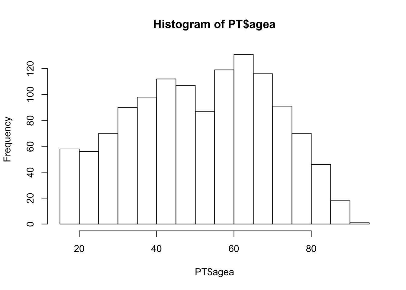
7.2 Two continuous variables
plot(PT$eduyrs ~ PT$agea)
abline(v=mean(PT$agea, na.rm=T), col="red")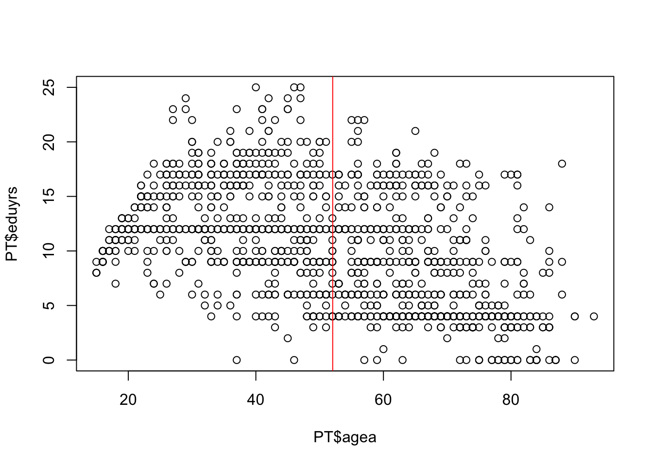
7.3 Categorical and continuous variable
boxplot(as.vector(PT$eduyrs) ~ PT$big.city)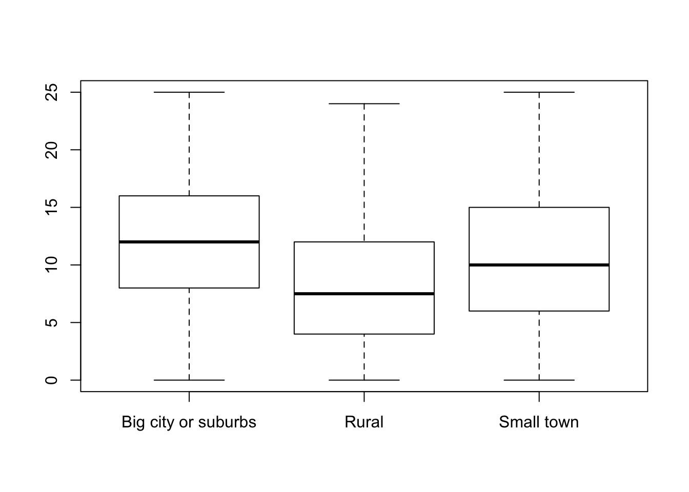
7.4 Math functions
curve(2*x + 1/sqrt(x), col="red")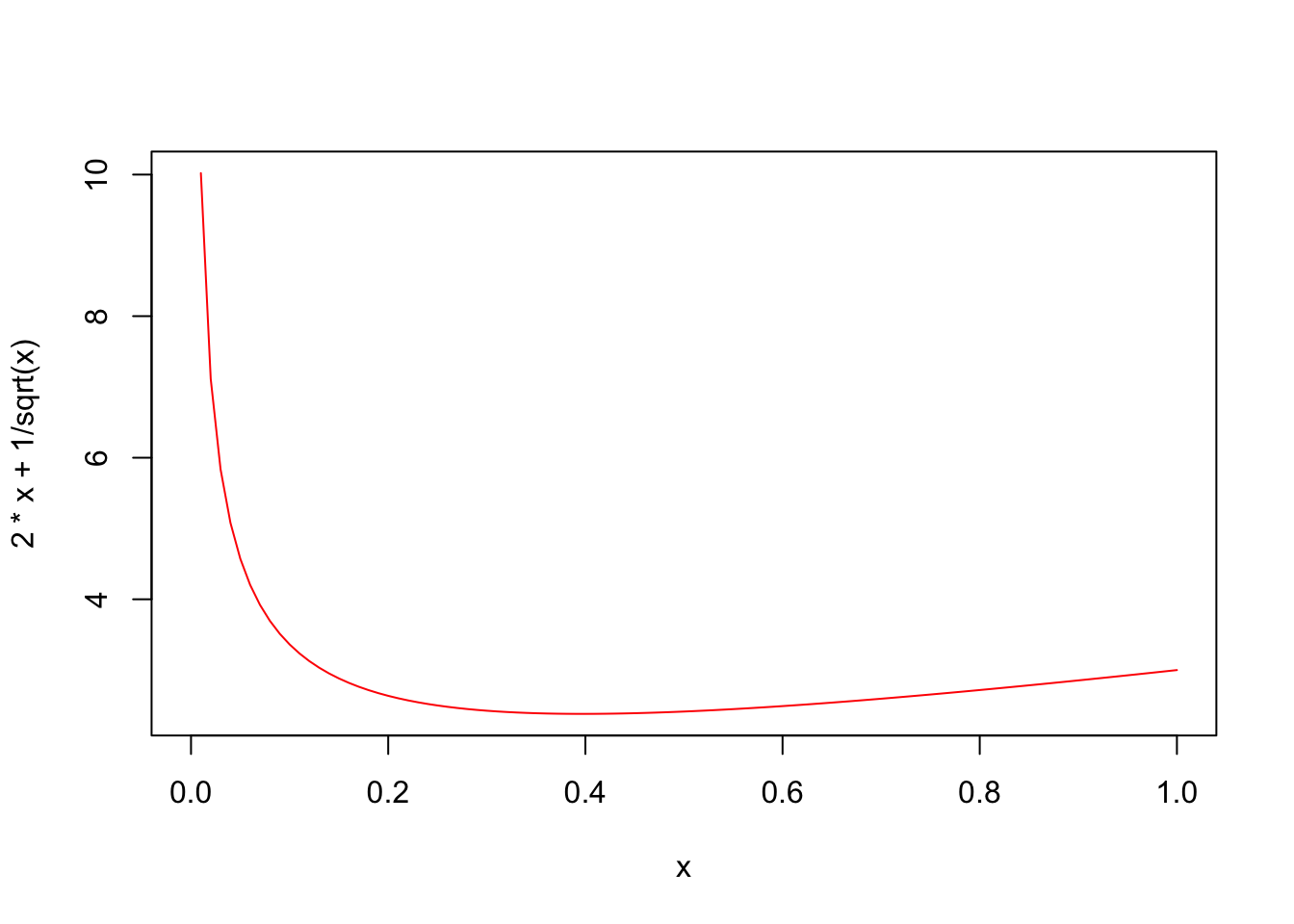
8 📤 Exporting tables and plots
There are many ways and it heavily depends on what you are going to do with these tables and plots.
8.1 Create an MS Word document
Directly generate a new MS Word document and add table:
library(officer)

cross.tab <- prop.table(table1,margin=2)

table.for.export <- as.data.frame.matrix(cross.tab)

d <- read_docx() #generate an empty Word document

d.appended <- body_add_table(d,                       # the empty doc object
                             table.for.export,        # data.frame to add
                             style = "table_template" # default style
                             )
d.appended <- body_add_par(d.appended,
                           "This is my table and some comments.",
                           style = "Normal"
                           )

print(d.appended, target = "data/mydocwithtable.docx") # write the file
[1] "/Users/maksimrudnev/Dropbox/DOCs/кафедра/Анализ и визуализация в R/2019_ISCTE_Workshop/data/mydocwithtable.docx"The generated file is here
8.2 Generate html file
It is a more universal way. You can open html documents in browser and then copy to MS Word.
Generate table -> export to html or LaTeX -> copy to MS Word.
library(stargazer)

stargazer(table.for.export,
          type = "html",
          out  ="data/table.html",
          summary = FALSE
          )
<table style="text-align:center"><tr><td colspan="5" style="border-bottom: 1px solid black"></td></tr><tr><td style="text-align:left"></td><td>Big city or suburbs</td><td>Rural</td><td>Small town</td><td>NA</td></tr>
<tr><td colspan="5" style="border-bottom: 1px solid black"></td></tr><tr><td style="text-align:left">1</td><td>0.011</td><td>0.005</td><td>0.007</td><td>0</td></tr>
<tr><td style="text-align:left">2</td><td>0.020</td><td>0.039</td><td>0.033</td><td>0</td></tr>
<tr><td style="text-align:left">3</td><td>0.064</td><td>0.103</td><td>0.059</td><td>0</td></tr>
<tr><td style="text-align:left">4</td><td>0.287</td><td>0.326</td><td>0.259</td><td>0</td></tr>
<tr><td style="text-align:left">5</td><td>0.283</td><td>0.258</td><td>0.325</td><td>0</td></tr>
<tr><td style="text-align:left">6</td><td>0.331</td><td>0.256</td><td>0.313</td><td>1</td></tr>
<tr><td style="text-align:left"></td><td>0.004</td><td>0.013</td><td>0.005</td><td>0</td></tr>
<tr><td colspan="5" style="border-bottom: 1px solid black"></td></tr></table>
Resulting file is here: table.html
8.3 Generate Excel files
write.csv(table.for.export, file="data/exported.table.csv")Resulting file is here: exported.table.csv
9 ⭕️ Solutions
9.1 Solution 1
#1-2
4 + 400
[1] 404#3
myVector <- c(1,2,3)
#4
myVector10 <- myVector * 10
myVector10[1] 10 20 30#5
myVector[2]*10[1] 209.2 Solution 2
#1-2 Manual, or automated:

download.file(url = "https://maksimrudnev.com/learn/iscte2019/data/ESS8PT.sav", destfile = "ESS8PT.sav")

#3

install.packages("haven")
library("haven")
PT <- read_sav("ESS8PT.sav")

# Alternative - one-line solution

PT <- haven::read_sav("https://maksimrudnev.com/learn/iscte2019/data/ESS8PT.sav")


# 4
str(PT)9.3 Solution 3
sum(PT$agea, na.rm=TRUE)/length(PT$agea)[1] 52.04882sum(PT$impfree.reversed, na.rm=TRUE)/length(PT$impfree.reversed)[1] 4.709449sqrt(var(PT$agea, na.rm=TRUE))[1] 18.30046sqrt(var(PT$impfree.reversed, na.rm=TRUE))[1] 1.107962