Assignments
Assignment 1
- Install R and RStudio on your computer.
- Install packages “car” and “haven”.
If you have your own data:
- read it in R;
- create a subset by relevant variable (for example, participants younger than 25);
- recode one variable;
- compute means of one variable by each age (or any other) group;
- export the means to the Word table.
If you don’t have your own data, or don’t want to use it:
- download ESS portugal - 2017 datafile;
- read it in R;
- create a subset of participants younger than 25;
- recode variable
healthto make variableillhealthso that 1 would stand for “Very good”, and 5 for “Very bad”. - compute means of variable
illhealthin each type of settlement (variabledomicil); - create the data.frame contatining the means and export it to the Word table.
Collect all the questions for the next Thursday. Save the resulting code as an R script file and send to me (Maksim.Rudnev@gmail.com) before Wednesday, 30th.
Solution
# Red in
library('haven')
ess.data <-  read_sav(file= "data/ESS8PT.sav")

# Subset
ess.data.less25 <- ess.data[ess.data$agea < 25,]

# Recode
library('car')

ess.data.less25$illhealth <- Recode(ess.data.less25$health, "1 = 5; 2 = 4; 3 = 3; 4 = 2; 5 = 1; else = NA")

# Means by group

ill.health.by.domicil<- aggregate(ess.data.less25$illhealth, list(ess.data.less25$domicil), mean, na.rm = TRUE )


# Export
library("officer")
d <- read_docx() #generate an empty Word document

d <- body_add_table(d,
                   ill.health.by.domicil,
                   style = "table_template"
                   )

print(d,
      target = "data/ill_health_table.docx")
## [1] "/Users/maksimrudnev/Dropbox/DOCs/кафедра/Анализ и визуализация в R/2019_ISCTE_Workshop/data/ill_health_table.docx"Assignment 2 (for credit or feedback)
- Create a project and a new R script. Read in the data ESS8PT.sav
- Recode the level of education in Portugal
edlvdptto 7 categories. - Compute the analysis of variance using
healthas dependent variable and the recoded education level as independent. - Fit the linear regression model:
healthas dependent variable, age (agea), recoded education, and gender (gndr) as independent. - Run the model diagnostics, testing for multicollinearity and heteroscedastiity.
- Add interaction of age and gender.
- Export it as a single table using
stargazer. - Visualize relations between key variables with
ggplot2.
Make sure R script works without errors, format it for easy reading, and send me (Maksim.Rudnev@gmail.com) before Wednesday, February 5.
Solution
# Create a project and a new R script. Read in the data [ESS8PT.sav](data/ESS8PT.sav)
library('haven')
ess.data <-  read_sav(file= "data/ESS8PT.sav")

# Recode the level of education in Portugal `edlvdpt` to 7 categories.

library('car')
ess.data$edu.pt <- Recode(ess.data$edlvdpt,
                      "1 = '1 Nenhum';
                       2 = '2 Básico 1';
                      3:5 = '3 Básico 2-3';
                      6:10 = '4 Secundário/Cursos v 2,3,4';
                      11:13 = '5 Superior politécnico/universitário';
                      14:16 = '6 Pós-graduação ou Mestrado';
                      17 = '7 Doutoramento';
                      else = NA",
                      as.factor = T )

# - Compute the analysis of variance using `health` as dependent variable and the recoded education level as independent.

anova1 <- aov(health ~ edu.pt, ess.data)
summary(anova1)
## Df Sum Sq Mean Sq F value Pr(>F)
## edu.pt 6 183.6 30.599 48.71 <2e-16 ***
## Residuals 1252 786.5 0.628
## ---
## Signif. codes: 0 '***' 0.001 '**' 0.01 '*' 0.05 '.' 0.1 ' ' 1
## 11 observations deleted due to missingness# - Fit the linear regression model: `health` as dependent variable, age (`agea`), recoded education, and gender (`gndr`) as independent.
m1 <- lm(health ~ agea + edu.pt + gndr, ess.data)
summary(m1)##
## Call:
## lm(formula = health ~ agea + edu.pt + gndr, data = ess.data)
##
## Residuals:
## <Labelled double>: Subjective general health
## Min 1Q Median 3Q Max
## -2.42241 -0.39216 -0.04760 0.44510 2.79436
##
## Labels:
## value label
## 1 Very good
## 2 Good
## 3 Fair
## 4 Bad
## 5 Very bad
## 7 Refusal
## 8 Don't know
## 9 No answer
##
## Coefficients:
## Estimate Std. Error t value
## (Intercept) 1.68987 0.18194 9.288
## agea 0.01477 0.00141 10.469
## edu.pt2 Básico 1 0.06651 0.13232 0.503
## edu.pt3 Básico 2-3 -0.21899 0.13658 -1.603
## edu.pt4 Secundário/Cursos v 2,3,4 -0.35716 0.14060 -2.540
## edu.pt5 Superior politécnico/universitário -0.50919 0.14685 -3.468
## edu.pt6 Pós-graduação ou Mestrado -0.65399 0.14320 -4.567
## edu.pt7 Doutoramento -0.66114 0.24118 -2.741
## gndr 0.21287 0.04341 4.904
## Pr(>|t|)
## (Intercept) < 2e-16 ***
## agea < 2e-16 ***
## edu.pt2 Básico 1 0.615325
## edu.pt3 Básico 2-3 0.109086
## edu.pt4 Secundário/Cursos v 2,3,4 0.011194 *
## edu.pt5 Superior politécnico/universitário 0.000543 ***
## edu.pt6 Pós-graduação ou Mestrado 5.44e-06 ***
## edu.pt7 Doutoramento 0.006209 **
## gndr 1.06e-06 ***
## ---
## Signif. codes: 0 '***' 0.001 '**' 0.01 '*' 0.05 '.' 0.1 ' ' 1
##
## Residual standard error: 0.7545 on 1250 degrees of freedom
## (11 observations deleted due to missingness)
## Multiple R-squared: 0.2665, Adjusted R-squared: 0.2618
## F-statistic: 56.76 on 8 and 1250 DF, p-value: < 2.2e-16# - Run the model diagnostics, testing for multicollinearity and heteroscedasticity.
library("lmtest")
vif(m1)## GVIF Df GVIF^(1/(2*Df))
## agea 1.472042 1 1.213277
## edu.pt 1.489299 6 1.033749
## gndr 1.012502 1 1.006232bptest(m1)##
## studentized Breusch-Pagan test
##
## data: m1
## BP = 18.557, df = 8, p-value = 0.01742# - Add interaction of age and gender.
m2 <- lm(health ~ agea*gndr + edu.pt , ess.data)
summary(m2)##
## Call:
## lm(formula = health ~ agea * gndr + edu.pt, data = ess.data)
##
## Residuals:
## <Labelled double>: Subjective general health
## Min 1Q Median 3Q Max
## -2.44444 -0.39630 -0.04135 0.44757 2.79563
##
## Labels:
## value label
## 1 Very good
## 2 Good
## 3 Fair
## 4 Bad
## 5 Very bad
## 7 Refusal
## 8 Don't know
## 9 No answer
##
## Coefficients:
## Estimate Std. Error t value
## (Intercept) 1.815485 0.255521 7.105
## agea 0.012187 0.003943 3.090
## gndr 0.126868 0.130264 0.974
## edu.pt2 Básico 1 0.072921 0.132667 0.550
## edu.pt3 Básico 2-3 -0.210616 0.137126 -1.536
## edu.pt4 Secundário/Cursos v 2,3,4 -0.349156 0.141089 -2.475
## edu.pt5 Superior politécnico/universitário -0.499463 0.147533 -3.385
## edu.pt6 Pós-graduação ou Mestrado -0.644784 0.143835 -4.483
## edu.pt7 Doutoramento -0.653447 0.241483 -2.706
## agea:gndr 0.001658 0.002368 0.700
## Pr(>|t|)
## (Intercept) 2.02e-12 ***
## agea 0.002043 **
## gndr 0.330280
## edu.pt2 Básico 1 0.582656
## edu.pt3 Básico 2-3 0.124809
## edu.pt4 Secundário/Cursos v 2,3,4 0.013466 *
## edu.pt5 Superior politécnico/universitário 0.000733 ***
## edu.pt6 Pós-graduação ou Mestrado 8.04e-06 ***
## edu.pt7 Doutoramento 0.006903 **
## agea:gndr 0.483890
## ---
## Signif. codes: 0 '***' 0.001 '**' 0.01 '*' 0.05 '.' 0.1 ' ' 1
##
## Residual standard error: 0.7547 on 1249 degrees of freedom
## (11 observations deleted due to missingness)
## Multiple R-squared: 0.2667, Adjusted R-squared: 0.2615
## F-statistic: 50.48 on 9 and 1249 DF, p-value: < 2.2e-16# - Export it as a single table using `stargazer`.
library("stargazer")
stargazer(m1, m2, type = "html", out = "data/summary_table.html")Check out the output file summary_table.html
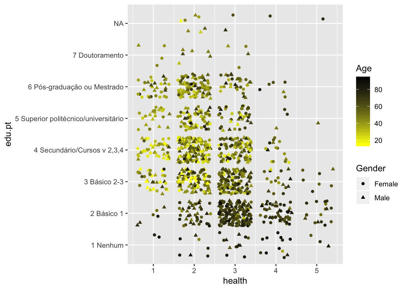
# - Visualize relations between key variables with `ggplot2`.
library("ggplot2")

ess.data$Gender <- Recode(ess.data$gndr, "1='Male'; 2='Female'", as.factor=TRUE)
ess.data$Age <- as.vector(ess.data$agea)

ggplot(ess.data,
       aes(x = Age,
           y = health,
           color = Gender))+
  geom_jitter()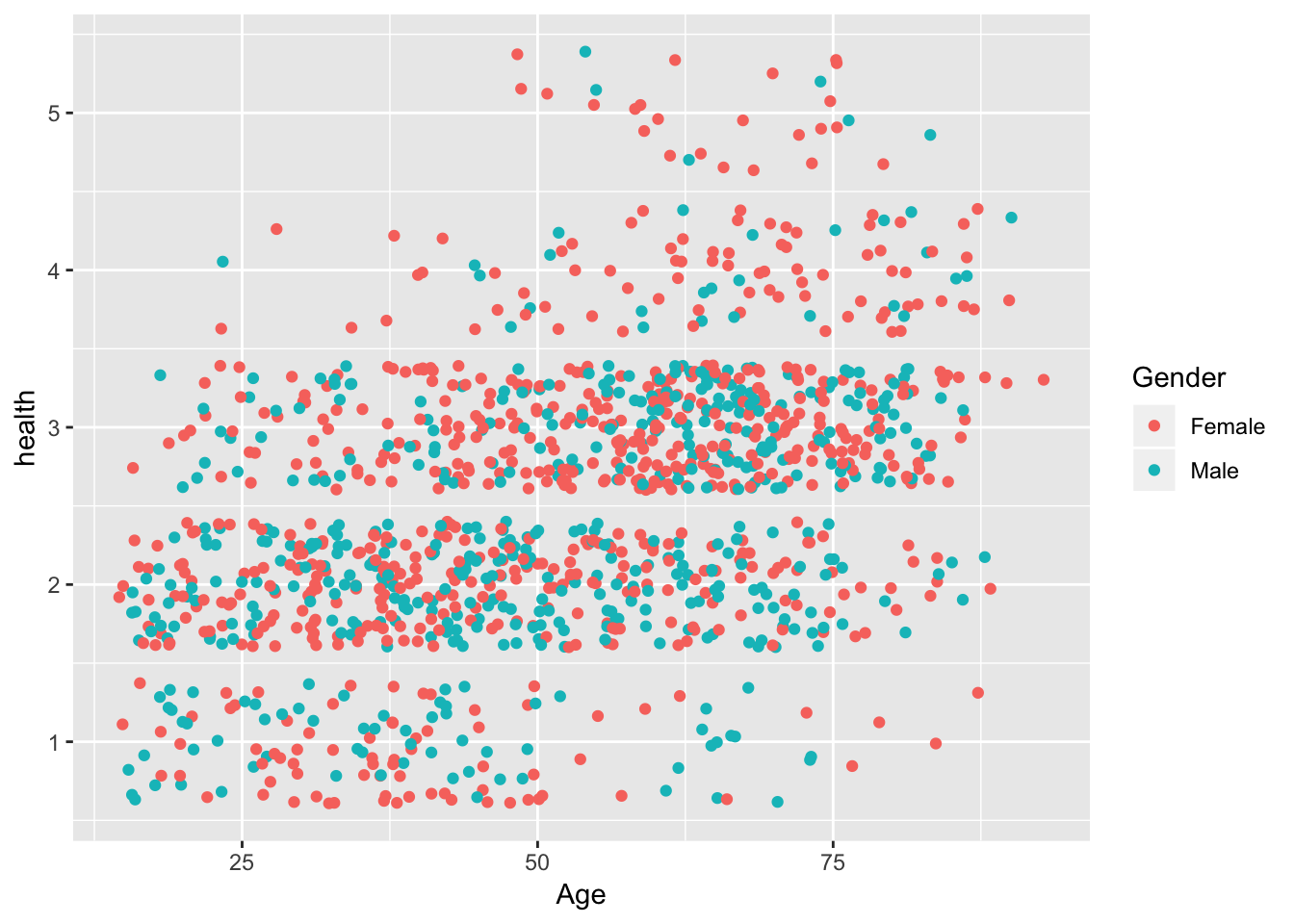
# OR

ggplot(ess.data,
       aes(x = health ,
           y = edu.pt,
           color = Age,
           shape = Gender))+
  geom_jitter()+
  scale_colour_gradient(low="yellow", high = "black")