
Content
indicators capture all theoretically relevant aspects of construct
 a.k.a. Occam’s Razor- entities should not be multiplied unnecesserily.
The simpler – the better. Unless otherwise is necessary.
If two models have the same fit to the data, the simpler one should be preferred.
Higher number of parameters automatically increases the model’s fit to the data, but decreases its fit to reality - the overfitting problem.
Data:
Model:
Is it reasonable to assume that a construct is measured without error?

The aim of factor analysis is to find parameters of latent variable(s), which explain all covariances between indicators via splitting variance of each indicator to the common and unique.
Every indicator is a linear combinatio of one or more latent factors and unique variance of indicator (residual/error).
because
The main purpose of PCA is to reduce dimensionality rather than to find latent variables. Example: image compression. To describe most of the pixels with only a few variables.
PCA doesn’t assume causal relations between variables, therefore:
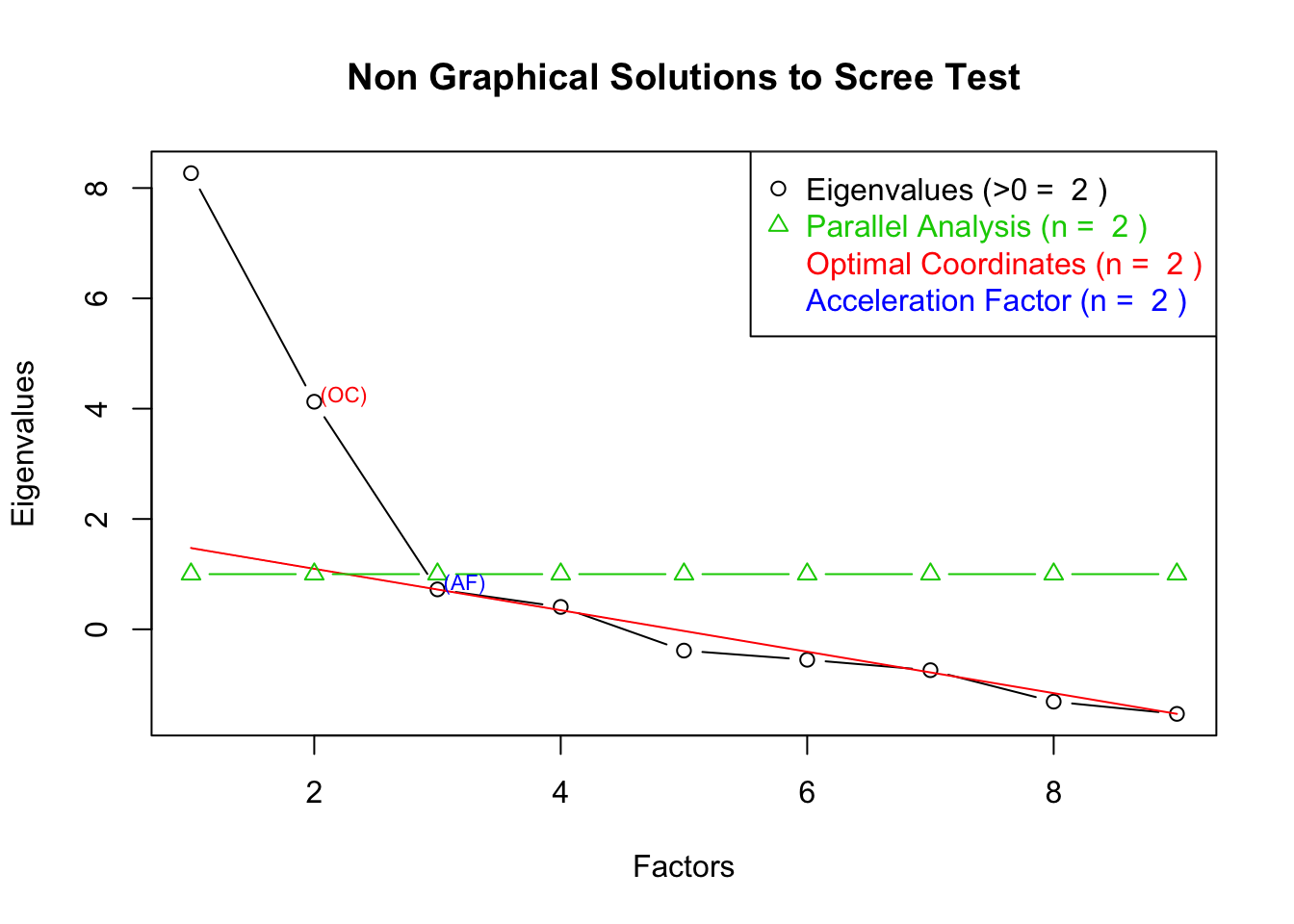
EFA provides guesses about underlying latent variable(s) by extracting common covariance (communalities). The main purpose of the first stage is to find a number (how many) factors.
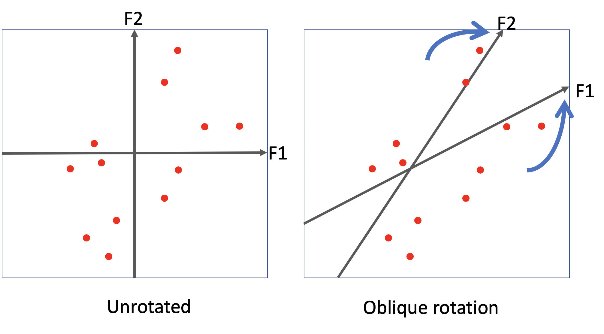
Factor rotation that simplifies the factor structure.
Results in a theory regarding the underlying latent variables and their structure.
Common criteria:
Rotated loadings (“oblimin” rotation)
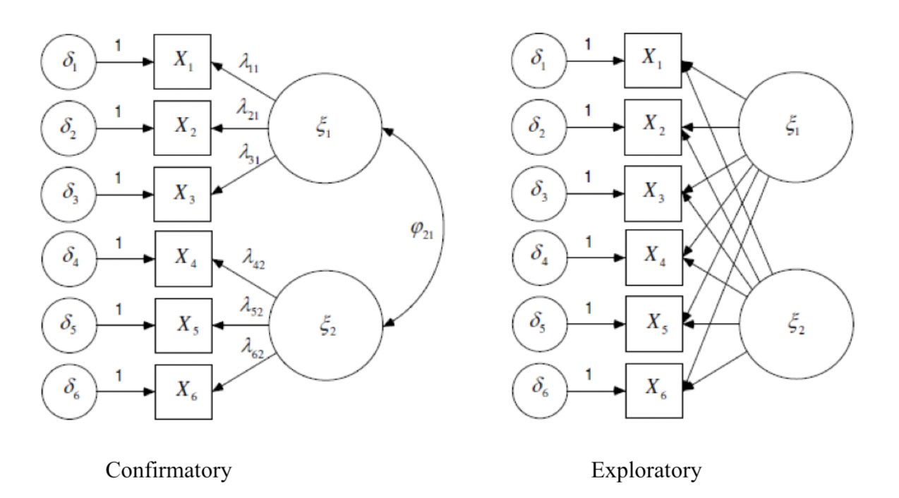
| Exploratory – EFA | Confirmatory – CFA |
|---|---|
| Usually no theory before analysis. | A priori theory is required. |
| Closely follows the data | Tests theory with the data |
| Aim is to descibe the data. | Aim is to test hypotheses. |
| Number of factors is unknown. | Number of factor is known from theory. |
| Applied at earlier stages of scale development | Applied later in scale development cycle, when the indicators are already known to manifest specific factors |
| All factor loadings are non-zero (harder to interpret) | Some factor loadings are fixed to zero |
All the common covariance between indicators is due to a latent factor.
Local independence - when the indicator residuals are not correlated, i.e. when the only common thing across indicators is a factor.
Quite often this assumption is unrealistic, because indicators have many sources of covariance, e.g.:
Variance of indicator =squared factor loading multiplied by factor variance + residual. \[ Var(y_1) = F.loading_{y_1}*F.loading_{y_1} * Var_{F_1} + Residual_{y_1} \]
Covariance between two indicators of single factor = simply a product of factor loadings and factor variance. \[ Covar_{y_1, y_2} = F.loading_{y_1}*F.loading_{y_2}*Var_{F}\] Covariance between two indicators of a single factor, with a covariance between residuals = product of two factor loadings, factor variance plus covariance of residuals. \[ Covar_{y1,y2} = F.loading_{y_1}*F.loading_{y_2}*Var_{F}+Covar_{Residuals(y_1,y_2)} \]
Covariance between two indicators of two different factors = product of corresponding factor loadings and covariance between factors. \[ Covar_{y1(F1),y3(F2)} = F1.loading_{y1} * F2.loading_{y3} * Covar_{F1,F2} \]
| ipadvnt | impfun | impdiff | |
|---|---|---|---|
| ipadvnt | 1.99 | 0.60 | 0.95 |
| impfun | 0.60 | 1.51 | 0.71 |
| impdiff | 0.95 | 0.71 | 1.76 |
Using formulas and parameter estimates on diagram, compute:
ipcrtivimpdiff and ipgdtim Answers
ipcrtiv = 1.5795862impdiff and ipgdtim = 0.6879641Identification of a model is a characteristic of a model (i.e. theory, not data) which allows to uniquely estimate (identify) parameters.
Example of non-identified model:
\[ x + y = 10 \]
\(x\) and \(y\) can take infinite number of values (e.g. 1 and 9, 5 and 5, 4.5 and 6.5, etc.) and the equation will still be true. Non-identification means there is not enough information in the model.
Example of identified model:
\[ x + 1 = 10 \]
Here, \(x\) can have only one unique value of 9.
The model \(x + y = 10\) has 2 unknown parameters and 1 known piece. Therefore, df= 1 - 2 = -1. This equation \(x + 1 = 10\) has 1 unknown parameter and 2 known pieces. Therefore, df = 2 - 1 = 1. Therefore this model is identified.
In CFA and other structural equation models the counted information is a number of unique elements in variance-covariance matrix of observed variables.
number of unique elements in variance-covariance matrix of observed variables : \[ N_{obs} = {k*(k+1)} / 2, \] where \(k\) is a number of observed variables. For example, for 4 observed variables, there are \[ N_{obs} = {4*(4+1)} / 2 = 10 \] ten unique pices of information.
\[ N_{parameters} = (N_{factors} * (N_{factors}+1))/2 + N_{obs.variables}*N_{factors} + N_{obs.variables} – N_{factors} \]
Parameters in CFA include:
Every factor in CFA should be given a metric to be identified.
Make sure that:
“Weakly identified” or “empirically underidentified” can occur in case of very high correlations between observed variables (~> 0.9).
Use an indicator which is the most reliable and most closely related to latent construct.
It sets the measurement unit of the latent variable.
-1 degrees of freedom
-1 degrees of freedom
To be able to compare the models, they must be nested.
The models are nested, if one can be derived from the other by either adding or removing parameters. Model with more parameters is called “full”, model with less parameters is called “reduced”.
In CFA, the typical nested models include:
Quality of the model is the similarity of estimated parameters to the true population parameters (given the model is correct). Impossible to check directly.
Model fit indicates the similarity between observed variance-covariance matrix and implied (i.e.predicted by model).
There are many (>50) fit indices. But a few are conventinally used: chi-square, CFI, TLI, RMSEA, SRMR.
| ipadvnt | impfun | impdiff | ipgdtim | ipcrtiv | impfree | |
|---|---|---|---|---|---|---|
| ipadvnt | 1.99 | 0.67 | 0.99 | 0.49 | 0.50 | 0.17 |
| impfun | 0.67 | 1.51 | 0.68 | 0.77 | 0.42 | 0.33 |
| impdiff | 0.99 | 0.68 | 1.76 | 0.66 | 0.68 | 0.38 |
| ipgdtim | 0.49 | 0.77 | 0.66 | 1.41 | 0.52 | 0.47 |
| ipcrtiv | 0.50 | 0.42 | 0.68 | 0.52 | 1.58 | 0.50 |
| impfree | 0.17 | 0.33 | 0.38 | 0.47 | 0.50 | 1.30 |
| ipadvnt | impfun | impdiff | ipgdtim | ipcrtiv | impfree | |
|---|---|---|---|---|---|---|
| ipadvnt | 1.99 | 0.60 | 0.95 | 0.58 | 0.57 | 0.33 |
| impfun | 0.60 | 1.51 | 0.71 | 0.77 | 0.43 | 0.25 |
| impdiff | 0.95 | 0.71 | 1.76 | 0.69 | 0.68 | 0.40 |
| ipgdtim | 0.58 | 0.77 | 0.69 | 1.41 | 0.41 | 0.24 |
| ipcrtiv | 0.57 | 0.43 | 0.68 | 0.41 | 1.58 | 0.50 |
| impfree | 0.33 | 0.25 | 0.40 | 0.24 | 0.50 | 1.30 |
| ipadvnt | impfun | impdiff | ipgdtim | ipcrtiv | impfree | |
|---|---|---|---|---|---|---|
| ipadvnt | 0.00 | -0.07 | -0.04 | 0.09 | 0.07 | 0.16 |
| impfun | -0.07 | 0.00 | 0.03 | 0.00 | 0.01 | -0.08 |
| impdiff | -0.04 | 0.03 | 0.00 | 0.03 | 0.00 | 0.02 |
| ipgdtim | 0.09 | 0.00 | 0.03 | 0.00 | -0.11 | -0.23 |
| ipcrtiv | 0.07 | 0.01 | 0.00 | -0.11 | 0.00 | 0.00 |
| impfree | 0.16 | -0.08 | 0.02 | -0.23 | 0.00 | 0.00 |
In just-identified models, χ2=0 always, but it means that we simply cannot estimate the model fit.
χ2 is sensitive to sample size. It is always large and significant (when N>1,000). For this reason, its interpretation is typically limited to small samples only.
\[\chi^2 = F_{max.lik.}(N-1) \] with a model degrees of freedom, where \(F_{max.lik.}\) - final value of maximum likelihood function; \(N\) - sample size.
Chi-square of factor [tested] model - compares observed variance-covariance matrix with the model-implied one.
Chi-square of baseline [independence] model - compares observed variance-covariance matrix with zeros. Measures probability that the data were generated by independence model. It’s usually very large and significant (and that’s ok).
Do not confuse these two!
Absolute fit, literally just the aggregated and standardized residuals.
Recommended values: <0.08
Recommended values: >0.90 or >0.95
Compares chi-squares of the model and of the imaginary “independence model” in which variables are unrelated to each other.
Weak null hypothesis, so CFI values are usually very high.
Theoretical range 0 : 1, where 0 is equality to “independence model”, and 1 is zero probability that the tested model is “independence model”.
\[ CFI = 1- \frac{\chi^2_{model}-df_{model}}{\chi^2_{independence}-df_{independence}}\]
TLI is very similar to CFI, though can be a bit higher than 1. Simulations have shown that this index might be more robust than the CFI.
\[ TLI = \frac{\frac{\chi^2_{independence}}{df_{independence}} - \frac{\chi^2_{model}}{df_{model}}}{ \chi^2_{independence}/df_{independence}-1 }\]
Parsimony-corrected fit index, i.e. corrects for the model complexity.
Recommended values: <0.08; <0.05.
Unlike other fit indices RMSEA has a confidence interval. The upper bound should not exceed 0.08.
PCLOSE – probability of RMSEA to be equal to 0.05; Pclose should be greater than .05.
It’s inversed index of fit, i.e. higher values mean worse fit.
Works better in larger samples.
\[ RMSEA = \sqrt\frac{\chi^2_{model} - df_{model}}{df_{model}*(N-1)} \]
well, at least three, preferably from different classes of fit indices to maximize insights drawing on their respective strengths.
Remember: every index has its benefits and downsides. If at least one fit index is beyond recomended values, the model cannot be accepted.
❗️ If the model fit is poor, estimated model parameters should not be taken seriously.
Chi-squre, CFI, TLI, and RMSEA are global fit indices, demonstrating fit of the whole model.
Standardized residuals may point to the problematic relations. Modification indicices can help finding missing parameters.
Preliminary estimates of estimates before they are actually included in the model.
A list of all the possible parameters not yet included in the model. Useful diagnostic information, for example:
NB. This works only for single parameters, that is, they change every time a new parameter is included in the model.
Simple difference between chi-squares of two nested models shows if adding/removing parameters significantly improved/decreased model fit to data.
If chi-square difference \(\chi^2_{difference} = \chi^2_{reduced} –\chi^2_{full}\) is significant, then full model has better fit. If it is insignificant, then reduced and full model have the same fit, so, following parsimony rule, the reduced model is preferred.
Difficult to test statistically, but larger CFI and TLI and smaller RMSEA and SRMR point to better models.
Information criteria - are just chi-squares with different adjustment by model complexity, sample size, and/or number of obserbed variables
Akaike Information Criterion - AIC \[ AIC = χ^2 - 2*df \]
Bayesian Information Criterion - BIC \[ BIC = χ^2+\log(N_{samp})*(N_{vars}(N_{vars} + 1)/2 – df) \]
The Sample-Size Adjusted BIC \[ SABIC = χ^2 +[(N_{samp} + 2)/24]*[N_{par}*(N_{par} + 1)/2 - df] \]
\(df\) - degrees of freedom, \(N_{vars}\) – number of variables in the model, \(N_{par}\) – number of free parameters on the model, \(N_{samp}\) – sample size.
The main focus of psychometrics
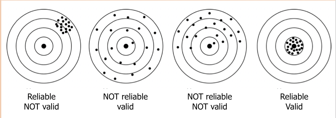
Degree to which latent variable scores are free of measurement error.
Common types of reliability:
Some researchers think DIF is a validity problem rather than reliability.
Higher values indicate higher consistency indicators, the share of the common variance in total variance of all indicators. \(\omega\) can be used only with indicators measured with the same scales.
\[ \omega_{McDonald} = \frac{(Sum~of~loadings)^2} {(Sum~of~loadings)^2+Sum~of~residuals +Covariance~of~residuals}\]
indicators capture all theoretically relevant aspects of construct
another instrument aimed to measure the same construct gives similar results
measure does not correlate to another construct to which it is not/weakly theoretically related
the measure is aligned with some other variable which is believed to be crucial for the construct. Criterion can usually be directly observed, or validly measured.
how well the measure can predict some theoretically relevant outcomes, e.g. ability to learn -> academic performance after 1 year at university
when the relations between latent construct (factor) and items (indicators) differ across groups
Increase in reliability can deteriorate validity, and vice versa.
Maksim wants a good measure of outgroup enmity. In the pilot questionnaire, he included five items on attitudes toward immigrants and 5 items on attitudes towards various social minorities. He found that Cronbach’s Alpha reliability coefficient was not high enough (only 0.5!). In the next version of the questionnaire, he replaced the second 5 items with more items on attitudes toward migrants. Reliability increased up to 0.85. Maksim is very happy now 🤓 But what happened to vthe alidity of the outgroup enmity scale?
second-order factor model
Second-order factors replace covariances of first-order factors. First-order factors are indicators of the second-order factors.