
Lecture 3. Multiple groups CFA
Multiple group CFA
CFA can be calculated using data from several groups simultaneously. It’s called Multi Group CFA (MGCFA).
MGCFA runs a single model, all the global fit statistics are estimated based on the data from all the groups.
Key feature - ability to constrain parameters across groups and test if they are equal.
Invariance models
Residuals are not shown here. Marker variable is used to identify the model.
Configural
Metric
Scalar
Levels and meaning of invariance
| Type of invariance | Meaning | Necessary conditions: equality of | Allows cross-group comparison of | ||
|---|---|---|---|---|---|
| Factor loadings | Intercepts | Residuals | |||
| No invariance | Differences in measurement are very large, the current instrument is not appropriate for comparisons | - | - | - | Can’t compare anything |
| Configural | Same construct is measured across groups, the same number of configuration of factors | Equal signs, same loadings and cross-loadings | - | - | Signs of correlations/regression coefficients |
| Metric | Construct is measured at the same scale (same units of latent variable), but the zero point differs across groups | + | - | - | Signs and magnitudes of correlations/regression coefficients |
| Scalar | Same units and same zero point of the latent variable scale | + | + | - | Everything above and factor means (latent means) |
| Partial scalar* | Same units and almost the same zero point of the latent variable scale | + | More than 2 are equal | - | Same as scalar, but more sceptical |
| Residuals | Indicators have the same quality across groups | + | + | + | Everything above and factor variances |
Testing measurement invariance with MGCFA
Configural, metric, and scalar invariance models are nested, so they can be compared with chi-square, CFI, TLI, and RMSEA.
Step 0. Before testing
Use theory to build a conceptually consistent and cross-culturally applicable measurement model. Run CFA separately in each group.
Step 1. Find a configural model
Run an MGCFA without cross-group constraints.
It should show a good fit (otherwise no further constraints can be tested).
The preferred method of identification is to use a marker indicator, because it is explicit. But there are other opinions.
Step 2. Run metric and scalar models
Run metric model: fix loadings across groups. Run scalar model: fix loadings and intercepts across groups.
Step 3. Compare the models
Compute differences between model fit indices using the chi-square difference test (if N is small) and/or use criteria proposed by Chen (2008): decrease in CFI of >0.01; increase in RMSEA >0.015 in model fit. That is, if \(\Delta CFI>\).01 and \(\Delta RMSEA>\).015 the invariance level should be rejected.
Chi Square Difference Test

            Df    AIC    BIC   Chisq Chisq diff Df diff Pr(>Chisq)
Configural 147 716083 719678  2295.1
Metric     227 716746 719656  3118.2      823.1      80  < 2.2e-16 ***
Scalar     307 725245 727470 11776.9     8658.8      80  < 2.2e-16 ***
Means      347 727582 729465 14193.6     2416.6      40  < 2.2e-16 ***
---
Signif. codes:  0 ‘***’ 0.001 ‘**’ 0.01 ‘*’ 0.05 ‘.’ 0.1 ‘ ’ 1

             CFI   ∆CFI   TLI   ∆TLI RMSEA ∆RMSEA  SRMR ∆SRMR
Configural 0.957        0.907        0.089        0.031
Metric     0.942 -0.015 0.919  0.012 0.083 -0.006 0.048 0.016
Scalar     0.768 -0.173 0.762 -0.157 0.143  0.059 0.092 0.044
Means      0.720 -0.048 0.746 -0.016 0.148  0.005 0.124 0.032
Step 3a. Celebrate and interpet parameters of interest
One way to compare latent means is to test for their equality, by first, fixing them to equality and then relaxing the constraint. If these two models fit the data equally well, then the means are indeed equal. This is alike one-way ANOVA and convenient with a large number of groups.

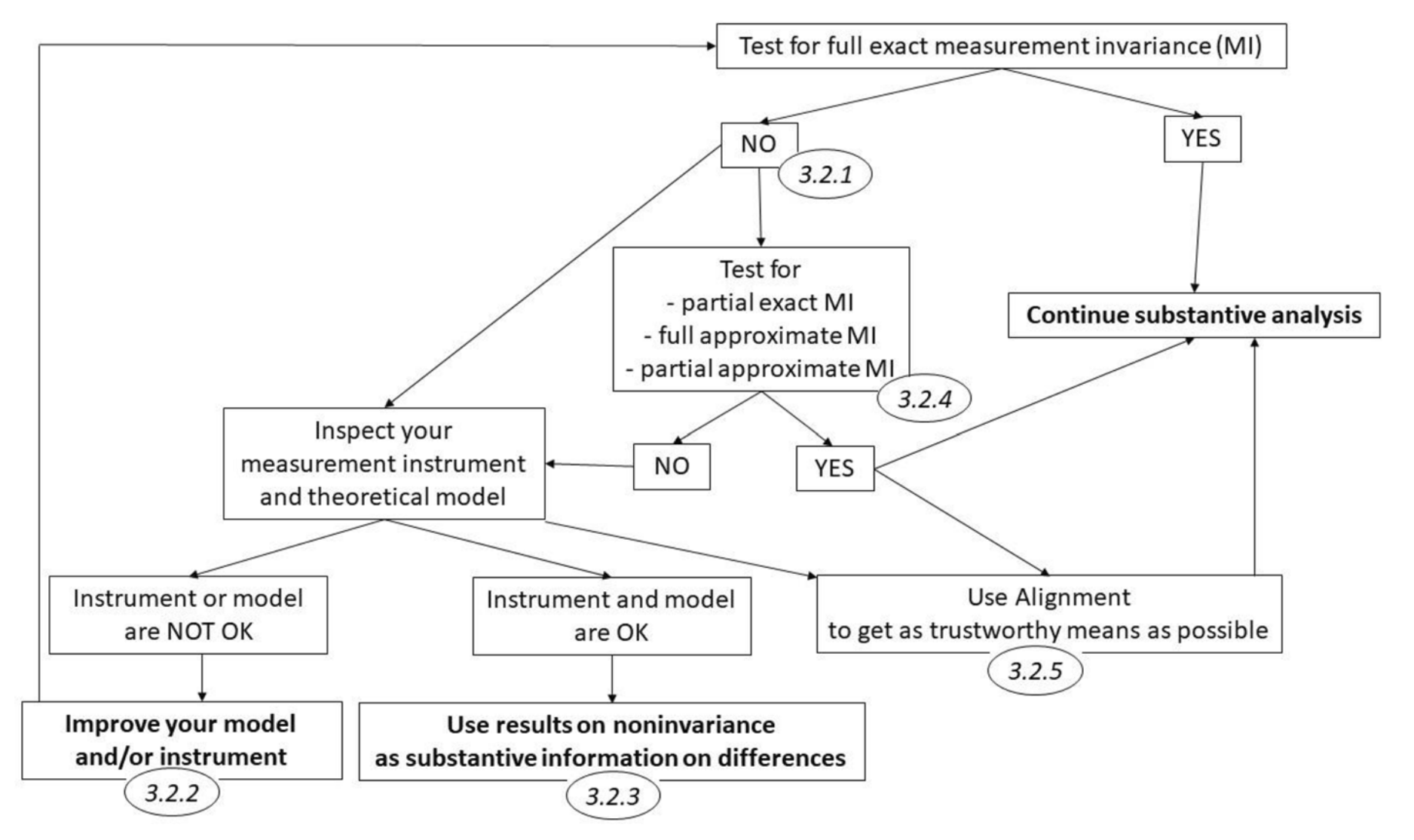
Step 3b. What if invariance was not found? (most often)
- misspecifications of the model across groups: check modification indices;
- small and theoretically grounded differences in models across groups are ok, e.g. residual covariance.
- see next lecture materials
- partial measurement invariance
- approximate measurement invariance
- alignment
- softer alternatives: target rotation, multidimensional scaling
or
- It’s uncomparable 🤷
- Try to explain the incomparability. It can be interesting by itself! See e.g. Trusinova 2014; Duelmer et al., 2013. There are advanced methods available, including multilevel SEM (but requires metric invariance) # Alternative strategy
It is possible to emply a top-down strategy, that is:
- begin with the most restricted model (scalar);
- if the fit is not ok, examine the modification indices and relax corresponding parameters;
- if fit is ok, still need to test metric and configural models to show that increase in the model fit is insignificantly small compared to the scalar model.
Real Examples from Papers
Davidov 2008
Trusinova 2014
Rudnev, in press
Problem
In European Social Survey, every questionnaire was translated independently from the original English questionnaire to a language used in a given country. In this way, six different translations into Russian appeared: in Russia, Estonia, Latvia, Lithuania, Ukraine, and Israel. None of the nine items measuring Self-Enhancement and Self-Transcendence had exactly the same wording.
Data
European Social Survey, round 4 and 5.
8,551 respondents, including 853 from Estonia, 538 from Latvia, 5,093 from Russia, and 2,067 from Ukraine. Israel and Lithuania were dropped because the sample sizes
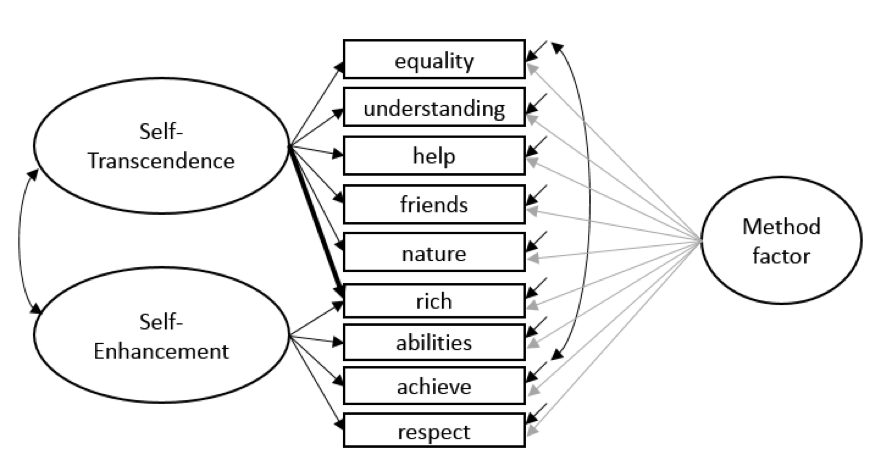
Table 1. Glorbal fit coeficients of MGCFA
| V1 | V2 | V3 | V4 | V5 |
|---|---|---|---|---|
| fit index | Configural MI model, loadings and intercepts are unconstrained, loadings of method factor are set to 1 for identification. | Metric MI model, the difference in factor loadings is set to 0, intercepts are not constrained. | Scalar MI model, difference in factor loadings are set to 0, intercepts are not constrained. | Partial scalar MI model, difference in factor loadings and intercepts is set to 0, intercepts of “respect” in Estonia and “success” in Russia are relaxed. |
| CFI | 0.969 | 0.963 | 0.939 | 0.957 |
| ΔCFI | - | 0.003 | 0.022 | 0.006 |
| TLI | 0.952 | 0.955 | 0.936 | 0.954 |
| RMSEA | 0.048 | 0.047 | 0.055 | 0.047 |
| ΔRMSEA | - | 0.001 | 0.008 | 0 |
| PCLOSE | 0.824 | 0.947 | 0.002 | 0.949 |
| SRMR | 0.036 | 0.044 | 0.051 | 0.046 |
| SABIC | 226380 | 226385 | 226694 | 226392 |
Wordings
Table 2. Original item wordings
Success - Being very successful is important to her/him. She/He hopes people will recognise her/his achievements.
Back translations:
- Estonia: “very mportant to be successful / people embrace their achievements”
- Latvia: “important to be successful / people embrace”
- Russia: “important to be
verysuccsessul” - Ukraine: “very impotrant to be successful”
Respect - It is important to her/him to get respect from others. She/He wants people to do what she/he says.
Back translations:
- Estonia: “…wants people
to obeyher/him and do the way she/he says” - Latvia: “…wants people to do what she/he says”
- Russia: “…wants people to do the way she/he says”
- Ukraine: “…wants people to do what she/he is saying”
Sample write-up of measurement invariance testing with MGCFA
The CFA model with the unconstrained factor loadings and intercepts is shown in Figure 1. Two CFA’s were conducted for group 1 (\(\chi^2=\); p=, CFI=; TLI=; RMSEA=), and group 2 (\(\chi^2=\); p=, CFI=; TLI=; RMSEA=), separately. Next, we tested for measurement invariance, see Table 1 for the fit indices. Model X has the lowest AIC/BIC value and therefore the best trade-off between model fit and model complexity. The other fit indices of Model X indicated a good fit. Compared to the group 2, group 1 appeared to have a significantly lower mean factor score (∆M=; p=).
van de Schoot et al., 2013. Checklist for measurement invariance
Or another, less generic write-up:
A factor model with two factors, LOVE-TO-LIVE and HATE-TO-DIE, each indicated by 4 items, was derived from the theory of COMMON SENSE and tested in the pilot sample. A test with a cross-cultural sample was conducted in three steps.
First, we fitted the factor model to the pooled sample data. The model was identified using the marker variable method. We used indicator ADVENTURES as a marker of the first factor and BADTIME of the second, because these indicators have similar meanings across cultures and conceptually seem to be the best manifestations of the corresponding constructs. Global fit measures demonstrated a good overall quality of the model (see Table 1), but modification indices suggested that adding a covariance between items FUN and GOODTIME would increase model fit. This covariation makes theoretical sense and therefore it was added to the model (see Table 1 for revised model fit). The two factors covaried significantly and positively. The final model is presented on Figure 1.
Second, we conducted a test of measurement invariance, the global fit indices are presented in Table 1. Configural and metric invariance models demonstrated a good fit to data, as well as scalar invariance model. An increase of 0.001 in CFI and decrease of 0.002 in RMSEA between configural and metric invariance models is within the range recommended by Chen (2008), therefore, the more constrained model showed comparable fit and given reasons of parsimony, the metric invariance model has fewer estimated parameters and therefore should be accepted. The invariant loadings are shown in the Figure 1. In contrast, the scalar invariance model was rejected, because the decrease in CFI and increase in RMSEA were greater than 0.05.
Third, we explored sources of the misfit in order to test a model of partial scalar invariance. An examination of modification indices suggested that relaxing intercept constraints for GOODTIME and BADTIME items would improve model fit. When both of intercepts were left to vary freely between groups, the difference in model fit between the metric invariance model and the partial scalar invariance model were within the recommended range, with the changes in CFI and RMSEA being 0.008 and 0.010 respectively. Therefore, we can accept the partial scalar invariance model. We can therefore compare the latent means between the ELFS and GOBLINS samples. The comparison of latent means showed that LOVE-TO-LIVE was significantly higher among ELFS, while there were no differences across groups by HATE-TO-DIE factor.
Table 1
| Df | BIC | Chisq | ∆Chisq | CFI | ∆CFI | RMSEA | ∆RMSEA | SRMR | ∆SRMR | |
|---|---|---|---|---|---|---|---|---|---|---|
| Pooled sample overall | 18 | 543.2 | 413.2 | 0.997 | 0.010 | 0.001 | ||||
| Configural | 36 | 533.5 | 492.3 | 0.960 | 0.011 | 0.010 | ||||
| Metric | 42 | 523.3 | 557.2 | 34.6* | 0.959 | 0.001 | 0.013 | 0.002 | 0.012 | 0.002 |
| Scalar | 48 | 580.1 | 659.1 | 108.3* | 0.908 | 0.051 | 0.070 | 0.057 | 0.050 | 0.038 |
| Partial scalar, intercepts of GOODTIME and BADTIME are unconstrained | 46 | 525.5 | 532.8 | 24.4* | 0.951 | 0.008 | 0.023 | 0.010 | 0.020 | 0.008 |
* The chi-square difference test is significant at p<0.05.