
Lecture 4 - Alternative and advanced ways to test for measurement invariance
Partial invariance in JASP
Tricky. Using the module SEM and writing a script 😱
lavaan syntax and SEM module of JASP
JASP -> Confirmatory factor analysis -> Additional Output -> Show lavaan syntax
# Factors
Factor1 =~ lambda11*pplfair + lambda12*pplhlp + lambda13*ppltrst

# Latent means
Factor1 ~ c(0,NA)*1
lavaan syntax conventions
| symbol | meaning | example |
|---|---|---|
=~ |
a new factor, its name on the right, its indicators on the left | MY_factor1 =~ indicator1 + indicator2 + indicator3 |
~1 |
intercept or mean | |
* |
Fix or constrain parameter to some value | My_factor =~ 1*my_indicator fixes the loading of my_indicator to 1; Factor1 ~ 0*1 constrains mean of Factor1 to 0. MY_factor1 =~ A*indicator1 + A*indicator2 constrains factor loadings of indicator1 and indicator2 to equality. |
c() |
Used to list constraints across groups | My_factor =~ c(1, A)*my_indicator fixes factor loading of my_indicator to 1 in the first group, and doesn’t fix it in the second group.My_factor =~ c(1, 1)*my_indicator fixes factor loading to 1 in both groups.My_factor =~ c(A, A)*my_indicator constrains factor loading in group 1 and group 2 to equality, forces them to be the same.my_indicator ~ c(0, NA)*1 fixes intercept of my_indicator to 0 in first group and freely estimate it in the second. |
NA |
“not available” in the sense the parameter is not fixed or constrained | My_factor =~ c(1, NA)*my_indicator - factor loading is fixed to 1 in the first group, but not fixed in the second. |
Resources
- JASP overview of SEM module: https://osf.io/xkg3j/
- lavaan homepage, with more examples of syntax: http://lavaan.ugent.be/tutorial/groups.html
Extra short intro to R lavaan
Step 1. Download R and Rstudio
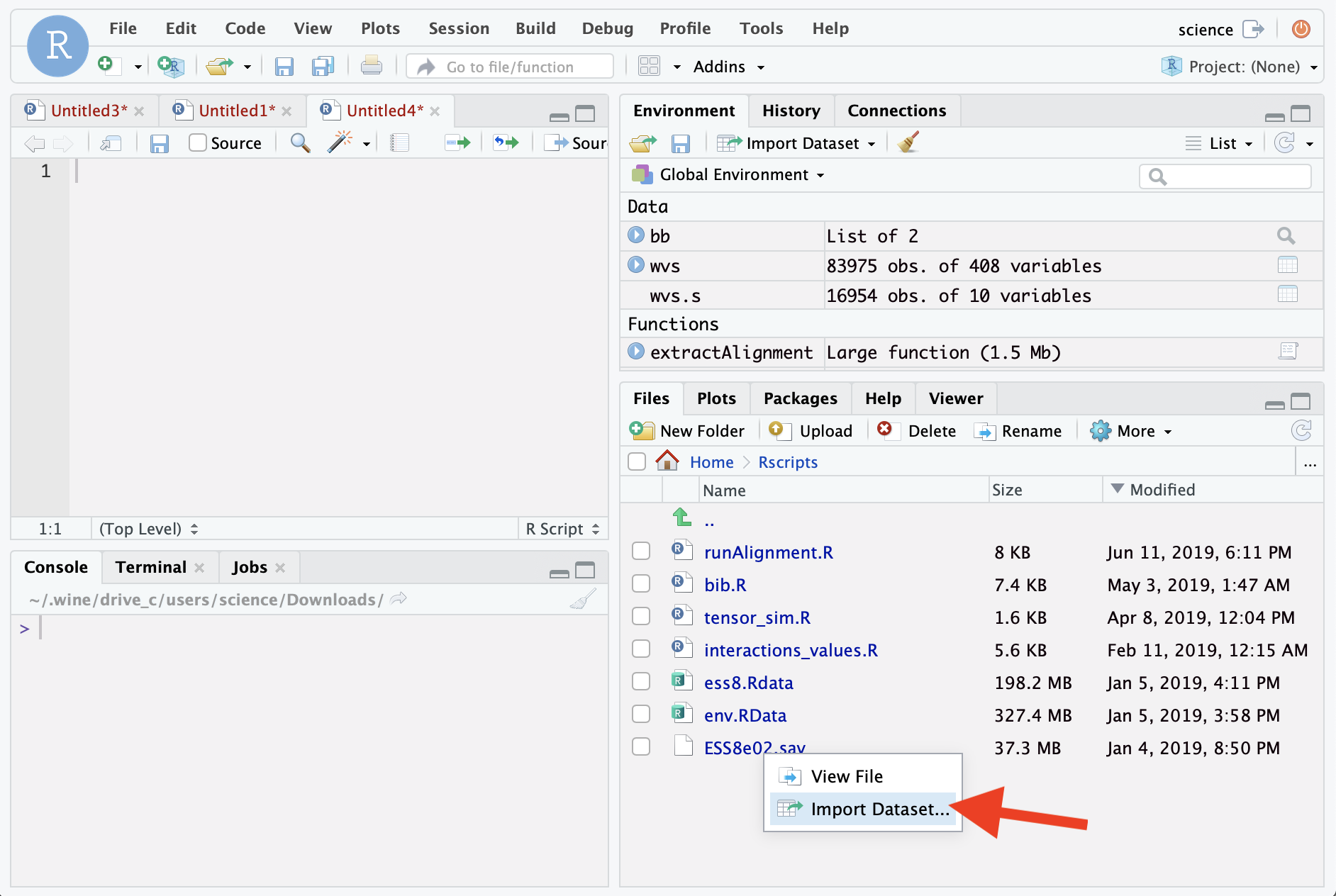
Step 2. Open the data
Step 3. Install and run “lavaan”
Add the lines in the ‘Source’ window. 
install.packages("lavaan")
library("lavaan")
To run the lines, select them and click “Run” button.
Step 4. Filter or modify data, if needed
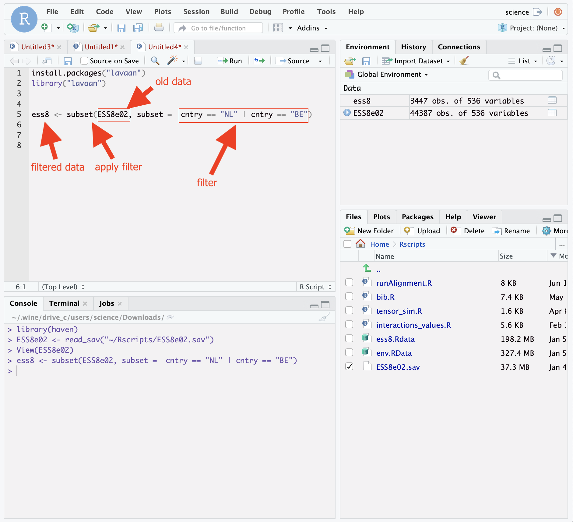
ess8 <- subset(ESS8e02, subset = cntry == "NL" | cntry == "BE")And run the line.
Step 5. Write the disirable “lavaan” code of the model
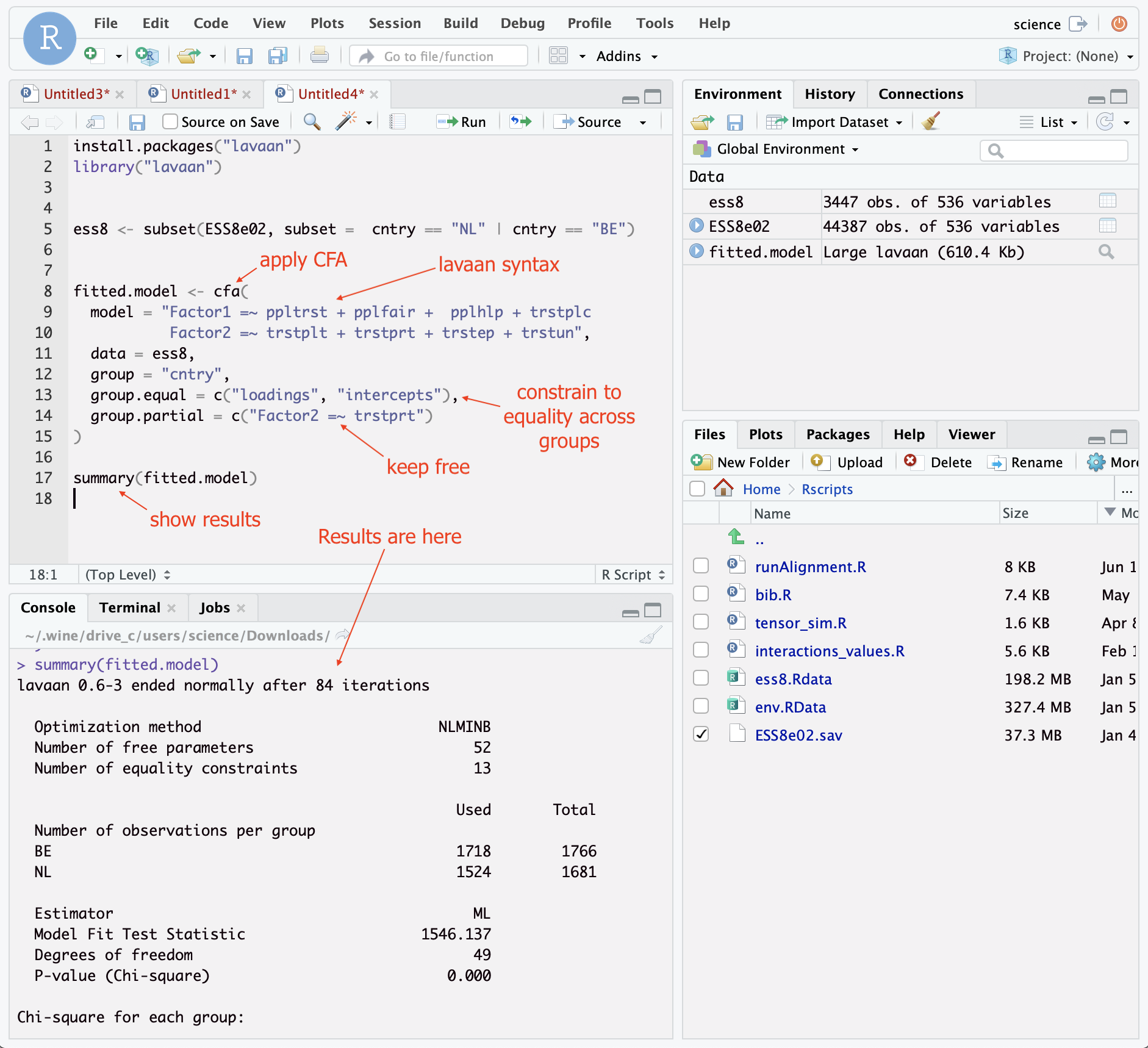
fitted.model <- cfa(
  model = "Factor1 =~ ppltrst + pplfair +  pplhlp + trstplc
           Factor2 =~ trstplt + trstprt + trstep + trstun",
  data = ess8,
  group = "cntry",
  group.equal = c("loadings", "intercepts"),
  group.partial = c("Factor2 =~ trstprt")
)

summary(fitted.model)
More resources
- Intro to R online course https://www.datacamp.com/courses/free-introduction-to-r or straight to modeling https://www.datacamp.com/courses/statistical-modeling-in-r-part-1
DIF – in item response theory
Item response theory- a set of methods, alike factor analysis, but aimed at categorical (binary) data. It was developed primarily for educational tests of achievements and abilities, initially for “right” and “wrong” answers.
Opposed to classic test theory (e.g. Cronbach), as more nuanced and theoretically underpinned.
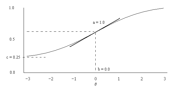
The indicators are not continuous, so the logistic function is used to create a continuous latent variable.
Most usual IRT models:
- Rasch model or 1-parameter model - the simplest;
- 3PL - three-parameter logistic model:
a- discrimination parameter [similar factor loading];b- difficulty parameter [similar to intercept];c- guessing parameter.
- Samejima’s graded response model; and partial credit models for ordinal indicators.
Source: Wikipedia
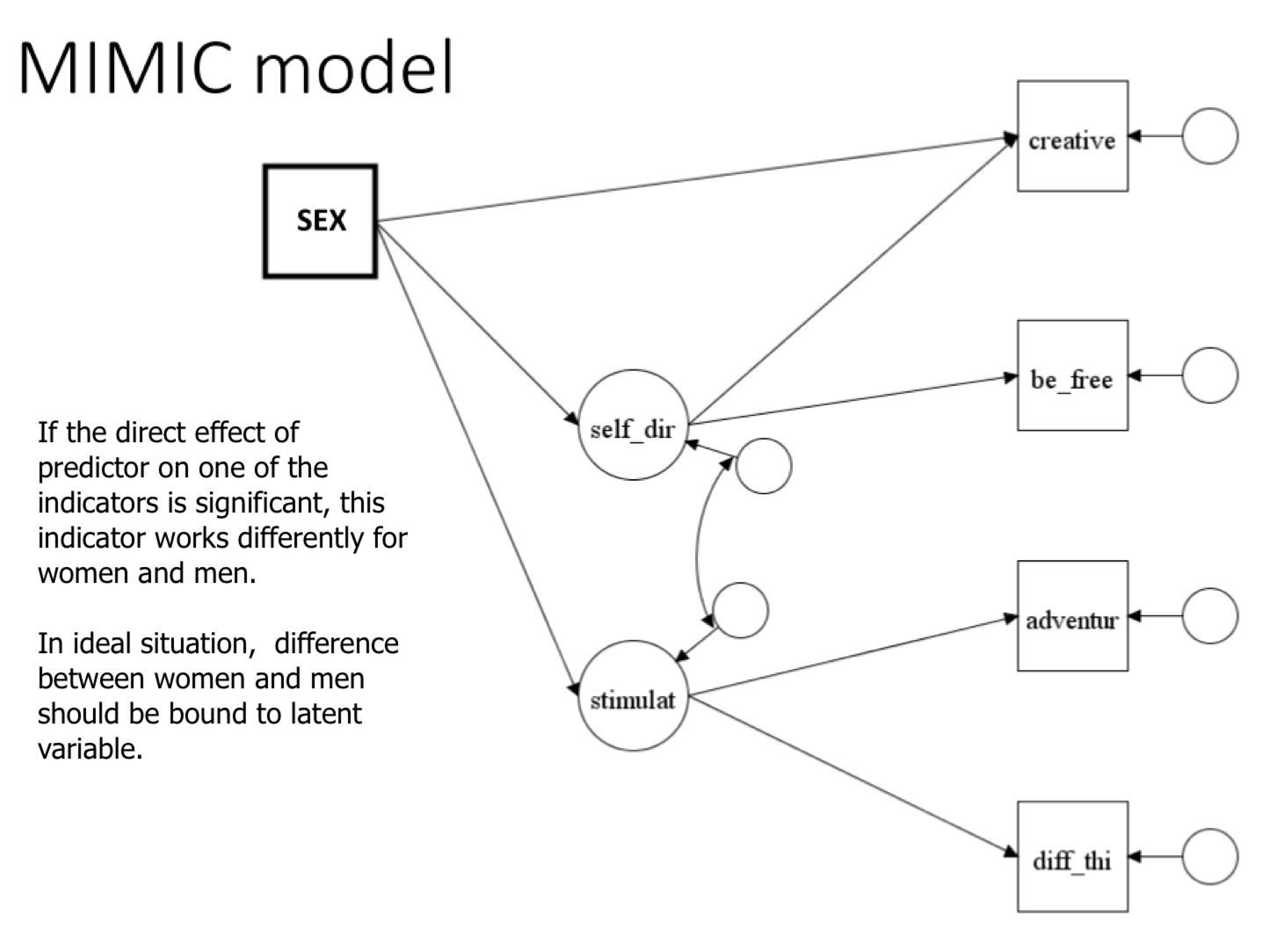
MIMIC - multiple indicators multiple causes
Appropriate for detecting non-invariant intercepts (but not factor loadings!). Conceptually appealing represention.
Approximate invariance
Based on scalar MGCFA model, but allows some wiggle space for loadings and intercepts.
Pros:
- Allows small differences in loadings and intercepts across groups.
- You can set an acceptable level of differences and check if it fits the data.
- Estimates an “approximate invariance”, typically higher invarinace level compared to the “exact” MGCFA.
- Uses Bayesian approach, which incorporates prior information about the subject into the model. Specifically, it includes 0 prior knowledge of the differences in factor loadings and intercepts across groups.
- Can be mixed with partial invariance approach.
- Very convenient when the data are noisy (many small cross-loadings or residual covariances).
Cons:
- Requires basic knowledge of Bayesian statistics;
- Sometimes it’s not clear if you have metric or scalar invariance;
- Time-consuming;
- Technical problems with model comparison;
- Available only with Mplus and R
blavaansoftware.
More explanations: van de Schoot et al., 2013
Alignment approach to measurement invariance
It gives more optimistic conclusions than the “exact” MGCFA test.
The alignment method can be used to estimate group-specific factor means and variances without requiring exact measurement invariance. Muthen & Asparouhov, 2013
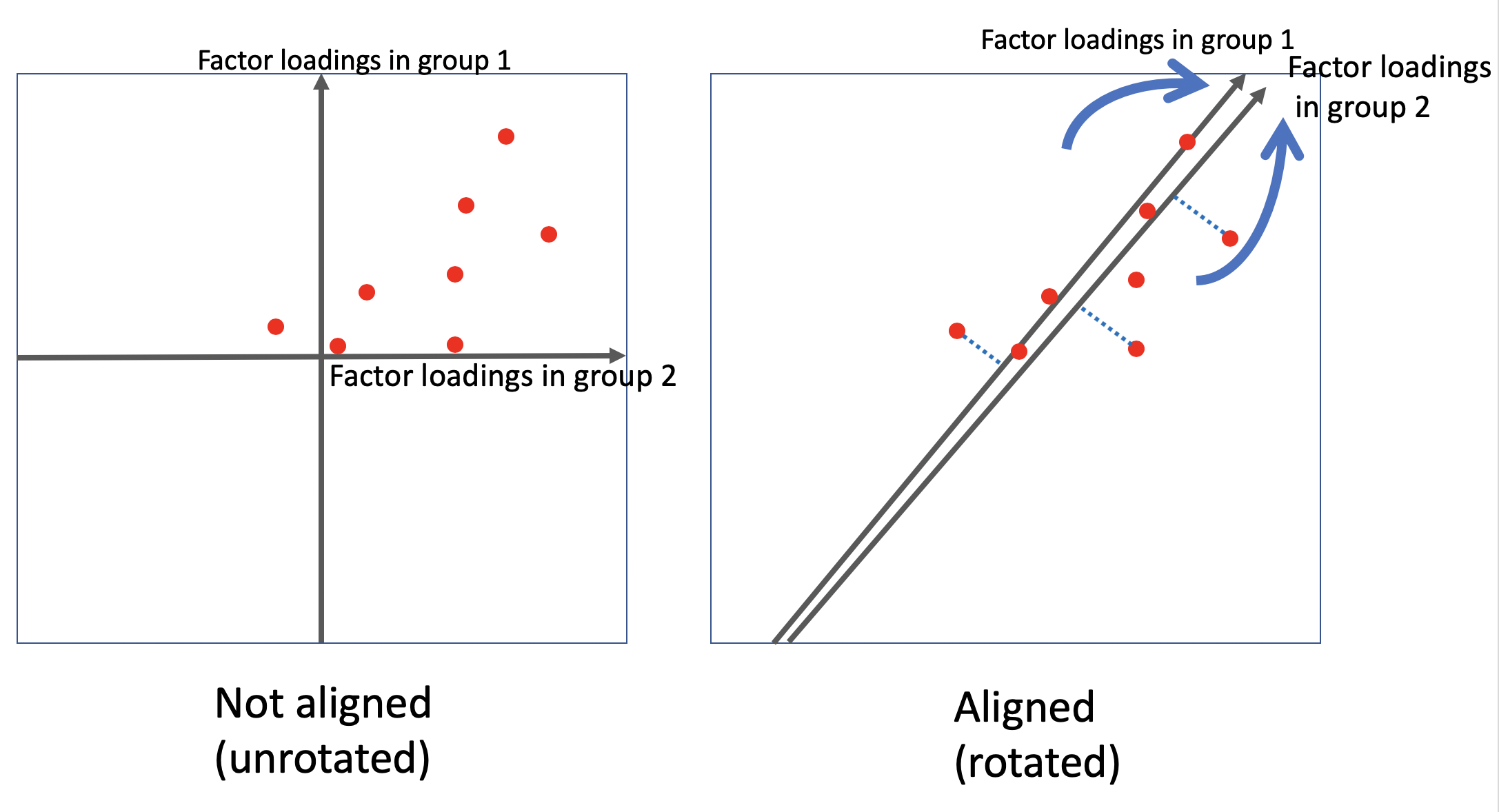
Consists of two stages:
- Configural model with free loadings and intercepts.
- Loadings and intercepts in different groups are “aligned” towards each other, alike rotation in EFA. It find an average solution for most groups and emphasizes the differences of outlier groups.
Assumptions:
- most parameters are invariant and a few or none are non-invariant;
- doesn’t work well with small number of groups (e.g. less than 10).
Pros and cons
| 😃 | ☹️ |
|---|---|
| - provides usually more optimistic results; | - requires many groups; |
| - gives a detailed info on every group and parameters non-invariance; | - requires Mplus licence |
| - allows comparison of latent means even when there is no full invariance; provides a direct comparison of latent means. | - sometimes doesn’t find invariance when it’s present |
Step-by-step tutorial
(requires Mplus software licence and basic knowledge of Mplus or R) https://maksimrudnev.com/2019/05/01/alignment-tutorial/
Target rotation
Similar to alignment, but with different steps.
- An exploratory factor analysis is run with a pooled sample (pancultural) or with a reference group. The factor loadings are extracted.
- For each group, exploratory factor analysis is run.
- Each group’s factor loadgins are rotated toward pancultural loadings.
Pros: - Convenient Tucker’s Phi coefficient shows the congruence between pancaultural loadings and rotated group-specific loadings; - employs more flexible EFA rather than CFA.
Cons: - test for structural/configural invariance only.
Available at R ccpsyc, or manually - at SPSS.
Other invariance tests
- dMACS to identify the degree/effect size of non-invariance, limited to single-factor models (Karl & Fischer 2019)
- Invariance across levels of continuous variables instead of groups, e.g. perception of ageism across ages (Bratt et al., 2018)
- Second-order factor invariance (Rudnev et al. 2018)
- Latent class (categorical latent variables) invariance here
- Explaining non-invariance with cultural characteristics (Davidov et al., 2012; 2018)
- Mixed models that search for sets of groups that have invariant parameters (de Roover, Vermunt, 2019)